Bayesian Analysis
- Bayesian inference is updating your beliefs after considering new evidence.
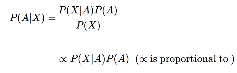
- We re-weight our prior beliefs after observing the evience and arrive at posterior probabilities
- As we gather an infinite amount of evidence, Bayesian results align with frequentist results. For large N, statistical inference is more or less objective. For small N inference is much more unstable, frequentist estimates have more variance and larger confidence intervals.
- Bayesian inference preserve the uncertainty that reflects the instability for a small N dataset.
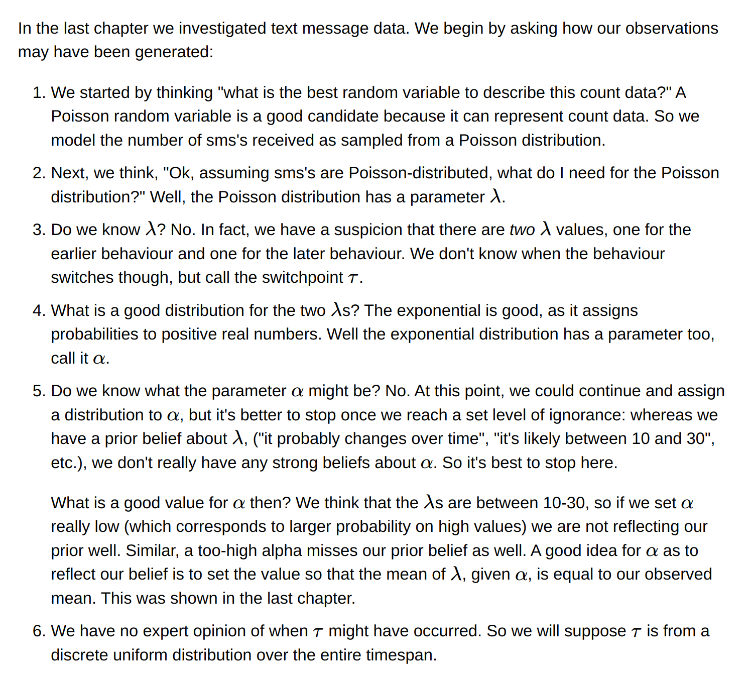
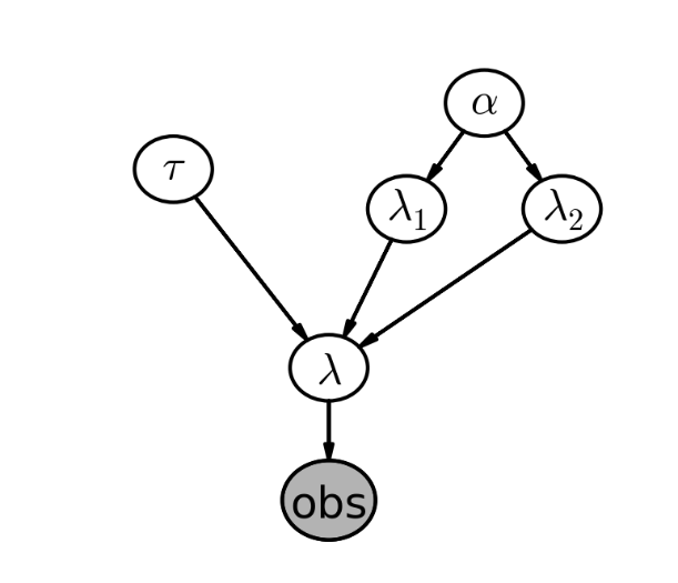
- A good starting point for Bayesian modeling is to think about how the data might have been generated.
- For getting the samples from posterior probability Monte Carlo Marko Chain (MCMC) algorithms are used
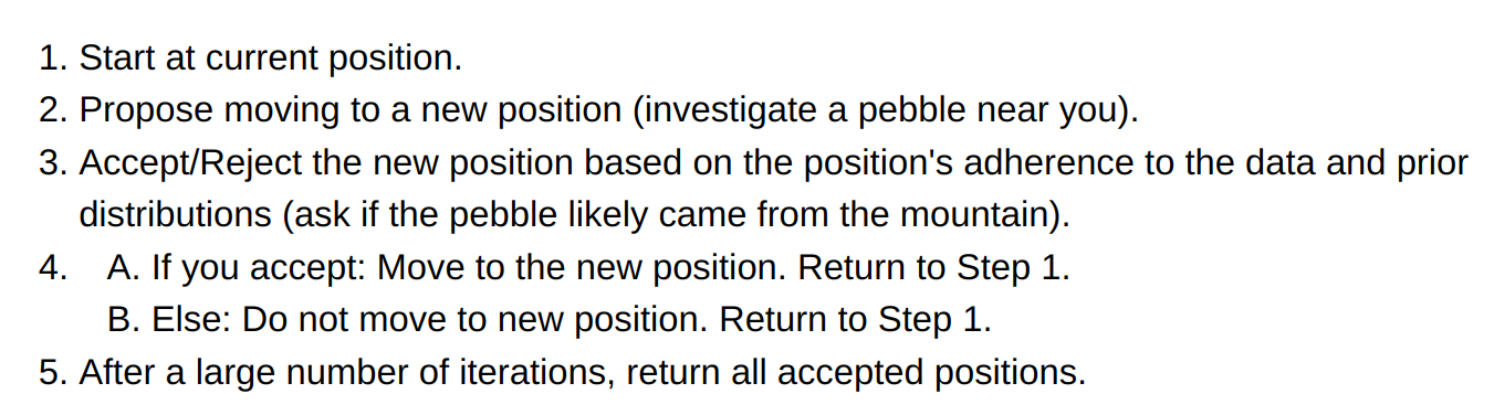
- In MCMC only the current location matters (memoryless)
- Laplace Approximations, Variational Bayes methods are also used to approximate the posterior.
- Metropolis sampling is used fElemwiseCategorical for categorical variables.
- A low auto-correlation between posterior samples are preferred
- Thinning - If we take every nth sample, we can remove some autocorrelation, with more thinning, the autocorrelation drops quicker. Higher thinning requires more MCMC iterations to achieve the same number of returned samples
- Law of large numbers - The average of a sequence of random variables from the same distribution converges to the expected value of that distribution. The law of large numbers is only valid as N gets infinitely large:never truly attainable.
- Small datasets should not be processed using the law of large numbers. We will encounter this problem when try to analyze subset of the data on some specific categories
- In Bayesian inference are computed using expected values. If we can sample from the posterior distribution directly, we simply need to evaluate averages.If further accuracy is desired, take more samples from the posterior.
- Bayesian inference also include loss functions. Instead of returning the average of posterior distribution, we can calculate minimum of the loss function to choose the estimate that minimized the expected loss. Minimum of the expected loss is called ‘Bayes action’
- In traditional ML it often happens that prediction measure and what frequentist methods are optimizing for are very different. For example in logistic regression trying to optimize cross entropy loss and trying to measure AUC, ROC, Precision etc. On the contrary, Bayes action is equivalent to finding parameters that optimize not parameter accuracy but an arbitary performance measure like loss functions, AUC, ROC, precision / Recall etc.
- Prior selected can be either objective or subjective. Objective prior is following the “principle of indifference” (all values are equally probable). Subjective prior is like adding our belief into the system ex. injecting domain knowledge.
- If the posterior does not make sense, then it means that the prior may not contain all the information and needs to be updated
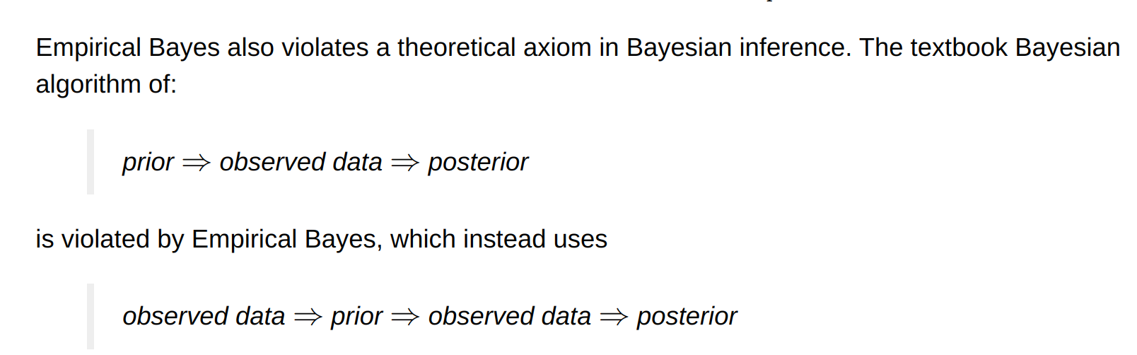
- Empirical Bayes combines frequentist and bayesian inference. Frequentist methods are used to find the prior’s hyperparameters and then proceed with bayesian methods. It was suggested not to use empirical bayes unless you have lots of data
Distributions useful for Priors
- Gamma distribution
- Wishart distribution - It is a distribution over all positive semi-definite matrices. covariance matrices are positive-definite, hence the Wishart is an appropriate prior for covariance matrices.
- Beta distribution is a generalization of uniform distribution
- A beta prior with binomial observations creates a beta posterior