import osmnx as ox
import matplotlib.pyplot as plt
import pandas as pd
import geopandas as gpd
import plotly.express as px
import keplergl
import warnings
warnings.filterwarnings(action='ignore')Visualizing Buildings in a location along with its Area
Import the required libraries
Plot the map for Pune
pune = ox.geocode_to_gdf("Pune, India")
pune.plot(edgecolor="0.2")
plt.title("Pune")
Text(0.5, 1.0, 'Pune')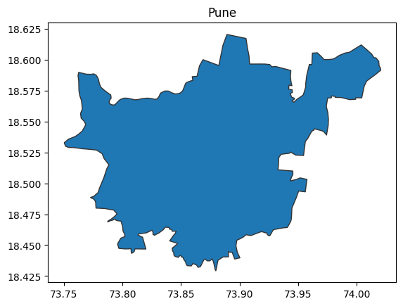
Plot your location on the Map
my_location = pd.DataFrame(
    {"location":["Baner"],
    "Longitude":[73.7747862],
    "Latitude":[18.578686]}
)my_location| location | Longitude | Latitude | |
|---|---|---|---|
| 0 | Baner | 73.774786 | 18.578686 |
my_location = gpd.GeoDataFrame(my_location,
                    crs = "EPSG:4326",
geometry=gpd.points_from_xy(my_location["Longitude"],my_location["Latitude"]))my_location| location | Longitude | Latitude | geometry | |
|---|---|---|---|---|
| 0 | Baner | 73.774786 | 18.578686 | POINT (73.77479 18.57869) |
ax = pune.plot(edgecolor="0.2")
my_location.plot(ax=ax,markersize=60,edgecolor="0.2",color='red')
plt.title("My Location in Pune")
Text(0.5, 1.0, 'My Location in Pune')
Get the Bike Routes for your location
bike_network = ox.graph_from_point(center_point=(18.5584546,73.7852182),dist=400,network_type='bike')
bike_network
<networkx.classes.multidigraph.MultiDiGraph at 0x7f3d9ae77f40>bike_network = (ox.graph_to_gdfs(bike_network, nodes=False)
.reset_index(drop=True)
.loc[:, ["name", "length", "geometry"]]
)
bike_network| name | length | geometry | |
|---|---|---|---|
| 0 | Gopal Hari Deshmukh Marg | 52.331 | LINESTRING (73.78688 18.56143, 73.78638 18.56145) |
| 1 | NaN | 127.050 | LINESTRING (73.78688 18.56143, 73.78683 18.560... |
| 2 | Pancard Clubs Road | 8.998 | LINESTRING (73.78638 18.56153, 73.78638 18.56145) |
| 3 | Gopal Hari Deshmukh Marg | 58.852 | LINESTRING (73.78638 18.56153, 73.78689 18.561... |
| 4 | Pancard Clubs Road | 8.998 | LINESTRING (73.78638 18.56145, 73.78638 18.56153) |
| ... | ... | ... | ... |
| 201 | NaN | 32.554 | LINESTRING (73.78206 18.55943, 73.78175 18.55946) |
| 202 | NaN | 47.738 | LINESTRING (73.78206 18.55943, 73.78204 18.55986) |
| 203 | NaN | 19.034 | LINESTRING (73.78206 18.55943, 73.78224 18.55944) |
| 204 | NaN | 32.554 | LINESTRING (73.78175 18.55946, 73.78206 18.55943) |
| 205 | NaN | 19.034 | LINESTRING (73.78224 18.55944, 73.78206 18.55943) |
206 rows × 3 columns
bike_network.plot()<AxesSubplot: >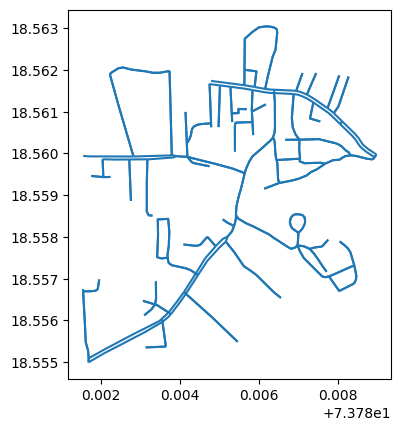
total_length = bike_network["length"].sum()
print(f"Total bike lane length: {total_length / 1000:.0f}km")
Total bike lane length: 16kmPlot Bike routes on the Map
import contextily as ctx

ax = (bike_network.to_crs("EPSG:3857")
         .plot(figsize=(10, 8), legend=True,
               edgecolor="0.2", markersize=200, cmap="rainbow")
     )
ctx.add_basemap(ax, source=ctx.providers.OpenStreetMap.Mapnik)  # I'm using OSM as the source. See all provides with ctx.providers
plt.axis("off")
plt.title("Baner")
Text(0.5, 1.0, 'Baner')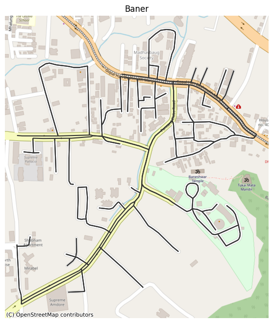
Get the building details in your area
tags = {'building':True}baner_buildings = ox.geometries_from_point(center_point=(18.5584546,73.7852182),dist=400,tags=tags)baner_buildings = baner_buildings.assign(label='Building Footprints').reset_index()(baner_buildings.head(10).T)| 0 | 1 | 2 | 3 | 4 | 5 | 6 | 7 | 8 | 9 | |
|---|---|---|---|---|---|---|---|---|---|---|
| element_type | node | way | way | way | way | way | way | way | way | way |
| osmid | 1432130601 | 264286363 | 359568513 | 359568520 | 359568545 | 359568551 | 359568562 | 359684077 | 359684097 | 359684099 |
| building | yes | yes | yes | yes | yes | yes | yes | yes | yes | yes |
| name | UBICS | Baneshwar Temple | NaN | NaN | NaN | NaN | NaN | NaN | NaN | NaN |
| geometry | POINT (73.7860015 18.5612441) | POLYGON ((73.7869388 18.5589314, 73.7869469 18... | POLYGON ((73.7889321 18.5605767, 73.7890453 18... | POLYGON ((73.7876847 18.56149, 73.7877554 18.5... | POLYGON ((73.78786 18.5613415, 73.7880387 18.5... | POLYGON ((73.7881551 18.559907, 73.7882733 18.... | POLYGON ((73.7828324 18.5618882, 73.782974 18.... | POLYGON ((73.7813494 18.5612504, 73.7814597 18... | POLYGON ((73.781994 18.5613356, 73.7821481 18.... | POLYGON ((73.7814951 18.5606079, 73.7817434 18... |
| nodes | NaN | [2699768401, 2699768402, 2699768403, 269976840... | [3642483644, 3642483643, 3642483641, 364248364... | [3642483654, 3642483653, 3642483648, 364248365... | [3642483649, 3642483647, 3642483645, 364248364... | [3642483640, 3642483639, 3642483637, 364248363... | [3642483660, 3642483659, 3642483657, 364248365... | [3643589874, 3643589877, 3643589867, 364358986... | [3643589882, 3643589883, 3643589873, 364358987... | [3643589826, 3643589830, 3643589824, 364358981... |
| amenity | NaN | place_of_worship | NaN | NaN | NaN | NaN | NaN | NaN | NaN | NaN |
| religion | NaN | hindu | NaN | NaN | NaN | NaN | NaN | NaN | NaN | NaN |
| addr:city | NaN | NaN | NaN | NaN | NaN | NaN | NaN | NaN | NaN | NaN |
| addr:postcode | NaN | NaN | NaN | NaN | NaN | NaN | NaN | NaN | NaN | NaN |
| addr:street | NaN | NaN | NaN | NaN | NaN | NaN | NaN | NaN | NaN | NaN |
| ways | NaN | NaN | NaN | NaN | NaN | NaN | NaN | NaN | NaN | NaN |
| type | NaN | NaN | NaN | NaN | NaN | NaN | NaN | NaN | NaN | NaN |
| label | Building Footprints | Building Footprints | Building Footprints | Building Footprints | Building Footprints | Building Footprints | Building Footprints | Building Footprints | Building Footprints | Building Footprints |
baner_buildings.name.fillna(value='not_known',inplace=True)baner_buildings.shape(255, 14)Visualize the buildings on the map
ax = (baner_buildings.to_crs("EPSG:3857")
         .plot(figsize=(10, 12),column="name",legend=True,
               edgecolor="0.2", markersize=200, cmap="rainbow")
     )
ctx.add_basemap(ax, source=ctx.providers.OpenStreetMap.Mapnik)  # I'm using OSM as the source. See all provides with ctx.providers
plt.axis("off")
plt.title("Baner")
Text(0.5, 1.0, 'Baner')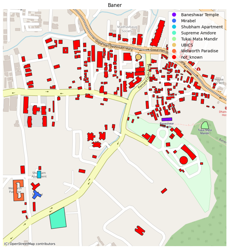
baner_buildings = baner_buildings.to_crs(epsg=3347)
baner_buildings = baner_buildings.assign(area=baner_buildings.area)baner_buildings= baner_buildings[['geometry','area']]Plot the buildings on the Map along with Area
baner_map = keplergl.KeplerGl(height=500)
baner_map.add_data(data=baner_buildings.copy(), name="Building area")
#baner_map.add_data(data=baner_buildings.copy(), name="height")
#baner_map
User Guide: https://docs.kepler.gl/docs/keplergl-jupyterbaner_map.save_to_html(file_name='first_map.html')Map saved to first_map.html!%%html
<iframe src="first_map.html" width="80%" height="500"></iframe>#from IPython.display import IFrame
#IFrame(src='first_map.html', width=700, height=600)