Converting Data from Raster to Tabular (Geometry) format

Import the libraries

import pandas
import osmnx
import geopandas 
import rioxarray
import xarray
import datashader as ds
import contextily as cx
from shapely import geometry
import matplotlib.pyplot as plt
import folium

import warnings
warnings.filterwarnings(action='ignore')

Download Geopackage

# URL for the geopackage
url = ("https://jeodpp.jrc.ec.europa.eu/ftp/"\
       "jrc-opendata/GHSL/"\
       "GHS_FUA_UCDB2015_GLOBE_R2019A/V1-0/"\
       "GHS_FUA_UCDB2015_GLOBE_R2019A_54009_1K_V1_0.zip"
      )
url

'https://jeodpp.jrc.ec.europa.eu/ftp/jrc-opendata/GHSL/GHS_FUA_UCDB2015_GLOBE_R2019A/V1-0/GHS_FUA_UCDB2015_GLOBE_R2019A_54009_1K_V1_0.zip'

Visualize the map

# Visualize the Map for Sao Paulo
p = f"zip+{url}!GHS_FUA_UCDB2015_GLOBE_R2019A_54009_1K_V1_0.gpkg"
fuas = geopandas.read_file(p)
sao_paulo = fuas.query("eFUA_name == 'São Paulo'").to_crs("EPSG:4326")

ax = sao_paulo.plot(alpha=0.5, figsize=(9, 9))
cx.add_basemap(ax, crs=sao_paulo.crs);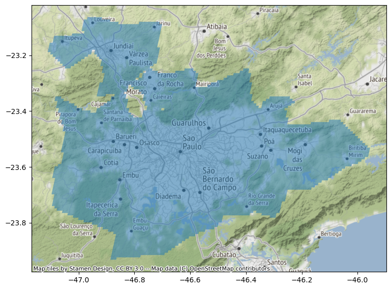

Download the population data

url = ("https://cidportal.jrc.ec.europa.eu/ftp/"\
       "jrc-opendata/GHSL/GHS_POP_MT_GLOBE_R2019A/"\
       "GHS_POP_E2015_GLOBE_R2019A_54009_250/V1-0/"\
       "tiles/"\
       "GHS_POP_E2015_GLOBE_R2019A_54009_250_V1_0_13_11.zip"
      )
url

'https://cidportal.jrc.ec.europa.eu/ftp/jrc-opendata/GHSL/GHS_POP_MT_GLOBE_R2019A/GHS_POP_E2015_GLOBE_R2019A_54009_250/V1-0/tiles/GHS_POP_E2015_GLOBE_R2019A_54009_250_V1_0_13_11.zip'

# Population data in raster format
%%time
p = f"zip+{url}!GHS_POP_E2015_GLOBE_R2019A_54009_250_V1_0_13_11.tif"
ghsl = rioxarray.open_rasterio(p)
ghsl

CPU times: user 35.6 ms, sys: 4.12 ms, total: 39.8 ms
Wall time: 7.12 s

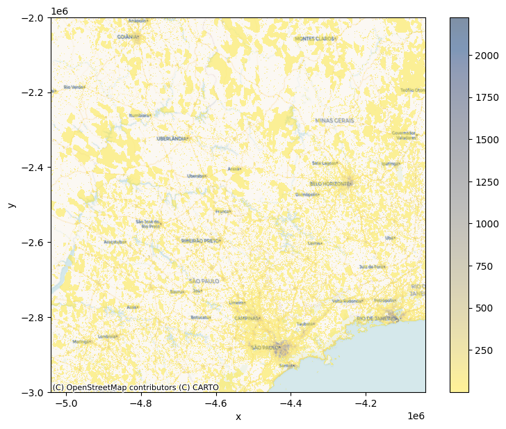
Visualize the population on raster data

cvs = ds.Canvas(plot_width=600, plot_height=600)
agg = cvs.raster(ghsl.where(ghsl>0).sel(band=1))

f, ax = plt.subplots(1, figsize=(9, 7))
agg.plot.imshow(ax=ax, alpha=0.5, cmap="cividis_r")
cx.add_basemap(
    ax, 
    crs=ghsl.rio.crs, 
    zorder=-1, 
    source=cx.providers.CartoDB.Voyager
)

# Clip the data for Sao Paulo
ghsl_sp = ghsl.rio.clip(sao_paulo.to_crs(ghsl.rio.crs).geometry.iloc[0])
ghsl_sp

/home/thulasiram/miniconda3/envs/geopy/lib/python3.9/site-packages/rasterio/features.py:290: ShapelyDeprecationWarning: Iteration over multi-part geometries is deprecated and will be removed in Shapely 2.0. Use the `geoms` property to access the constituent parts of a multi-part geometry.
  for index, item in enumerate(shapes):

out_p = “../data/ghsl_sao_paulo.tif” ! rm $out_p ghsl_sp.rio.to_raster(out_p)

Convert Raster to geometry

# Read the raster data
surface = xarray.open_rasterio("../data/ghsl_sao_paulo.tif")

# Convert raster to geometry
t_surface = surface.to_series()

t_surface.head()

band  y           x         
1     -2822125.0  -4481875.0   -200.0
                  -4481625.0   -200.0
                  -4481375.0   -200.0
                  -4481125.0   -200.0
                  -4480875.0   -200.0
dtype: float32

t_surface = t_surface.reset_index().rename(columns={0: "Value"})

t_surface.query("Value > 1000").info()

<class 'pandas.core.frame.DataFrame'>
Int64Index: 7734 entries, 3785 to 181296
Data columns (total 4 columns):
 #   Column  Non-Null Count  Dtype  
---  ------  --------------  -----  
 0   band    7734 non-null   int64  
 1   y       7734 non-null   float64
 2   x       7734 non-null   float64
 3   Value   7734 non-null   float32
dtypes: float32(1), float64(2), int64(1)
memory usage: 271.9 KB

type(t_surface)

pandas.core.frame.DataFrame

# Calculate the polygon based on resolution values
def row2cell(row, res_xy):
    res_x, res_y = res_xy  # Extract resolution for each dimension
    # XY Coordinates are centered on the pixel
    minX = row["x"] - (res_x / 2)
    maxX = row["x"] + (res_x / 2)
    minY = row["y"] + (res_y / 2)
    maxY = row["y"] - (res_y / 2)
    poly = geometry.box(
        minX, minY, maxX, maxY
    )  # Build squared polygon
    return poly

# Get the polygons
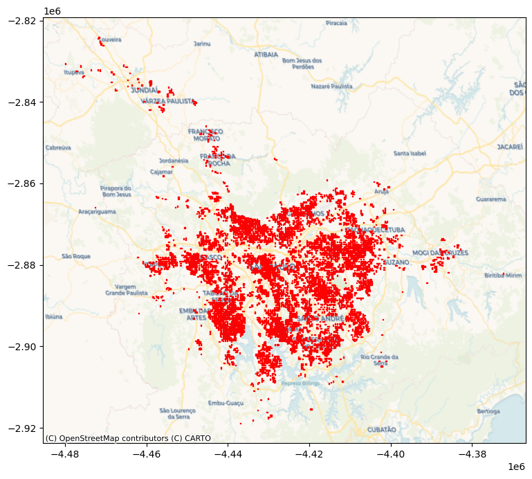
max_polys = (
    t_surface.query(
        "Value > 1000"
    )  # Keep only cells with more than 1k people
    .apply(  # Build polygons for selected cells
        row2cell, res_xy=surface.attrs["res"], axis=1
    )
    .pipe(  # Pipe result from apply to convert into a GeoSeries
        geopandas.GeoSeries, crs=surface.attrs["crs"]
    )
)

# Plot polygons on the map
ax = max_polys.plot(edgecolor="red", figsize=(9, 9))
# Add basemap
cx.add_basemap(
    ax, crs=surface.attrs["crs"], source=cx.providers.CartoDB.Voyager
)

Convert Geometry to Raster

new_da = xarray.DataArray.from_series(
    t_surface.set_index(["band", "y", "x"])["Value"]
)
new_da