Fitting functions to data
- Linear functions can be either concave or convex. when we take the maximum of linear functions, we are compensated with convexity
- If we have non-linear convex function, then the maximum of all the linear functions that stay below our function is exactly equal to it. This gives us a path to exploit the simplicity of linear functions when we have convex functions.
- For convex functions the global and local minima are same
- A non-linear function can be either convex or non-convex
- For non-convex functions with peaks, valleys and saddle points we run the risk of getting stuck at local minima
- Numerical method’s search for minimum happens on the ground level and does not search in the same space dimension as the landscape of the function is embedded in.
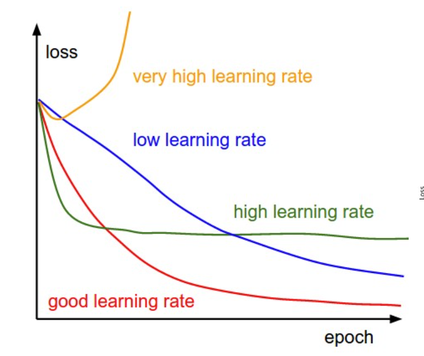
- It is important to locate, on ground level, a direction that quickly decreseas the function height and how far we can move in that direction on ground level (learning rate) while still decreasing the function height above us
Linear regression
- Analytic and numeric method exist for linear regression. For others analytic solution is difficult, so we depend on numeric methods

Logistic regression
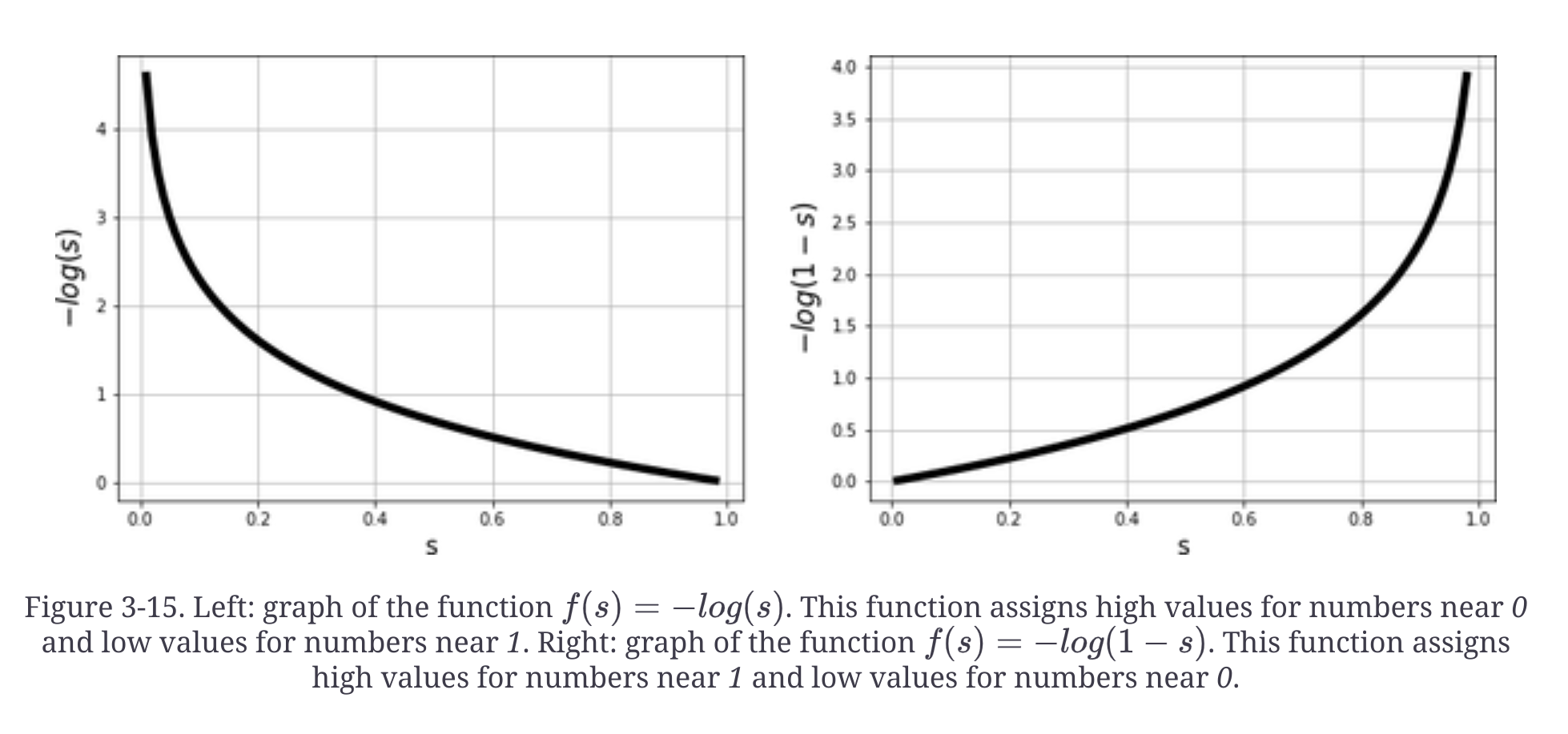
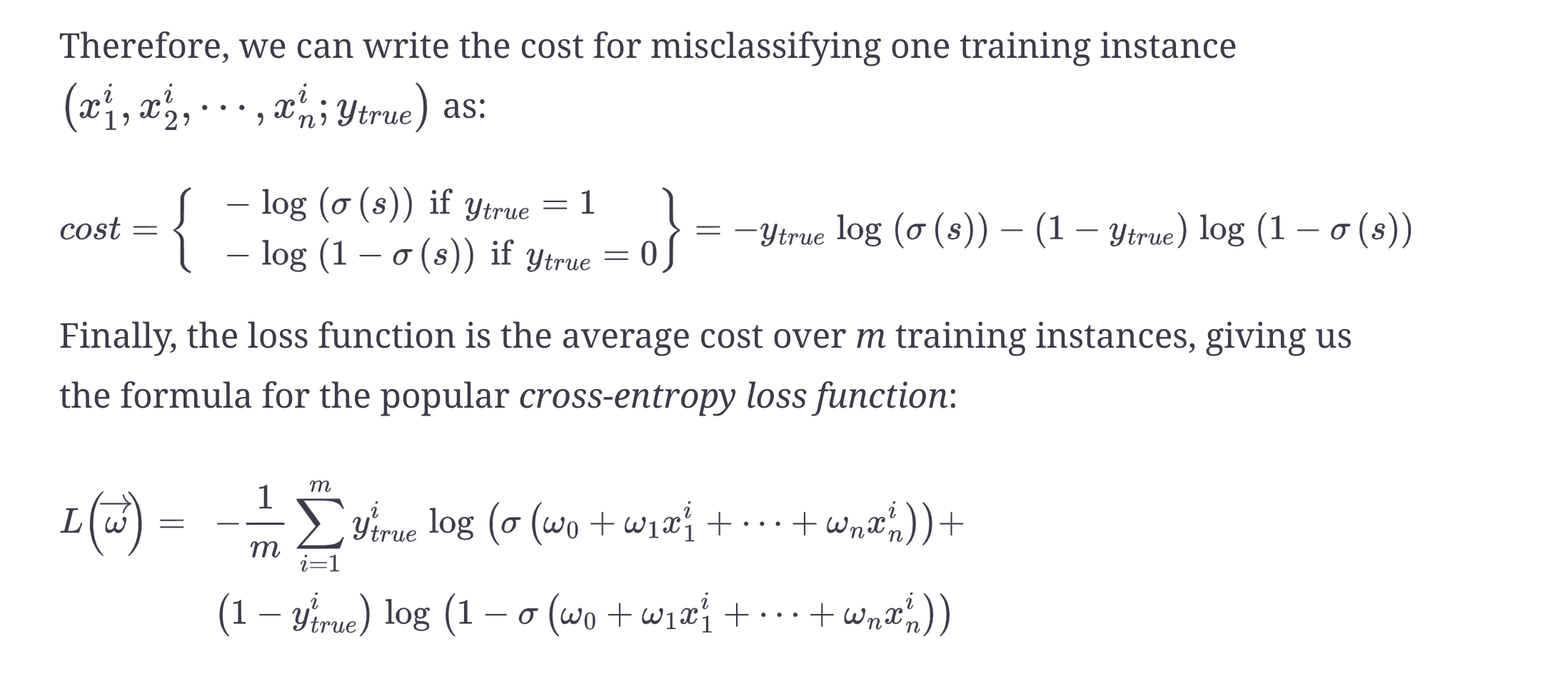
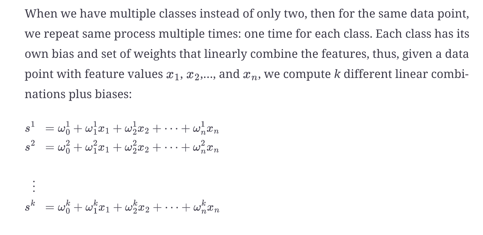
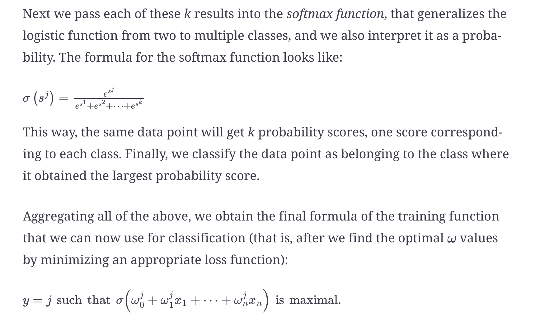
Multiclass logistic function

SVM
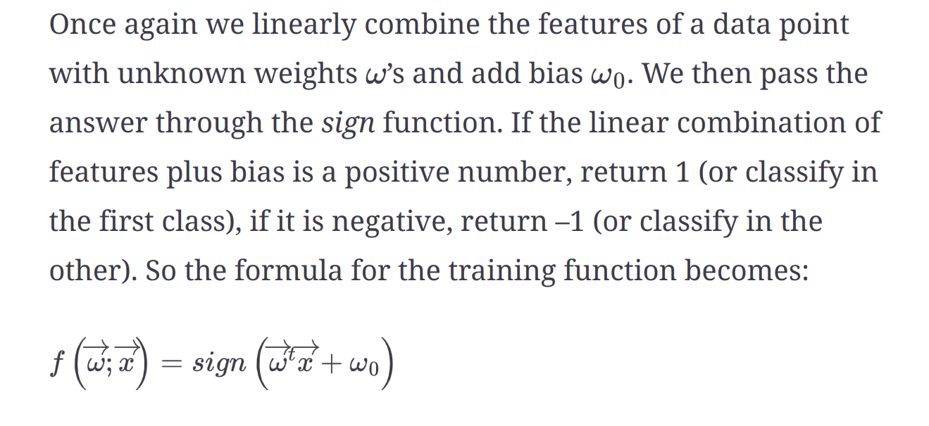
- Seek to separate a labeled data using widest possible margin
- An optimal highway of separation instead of thin line of separation
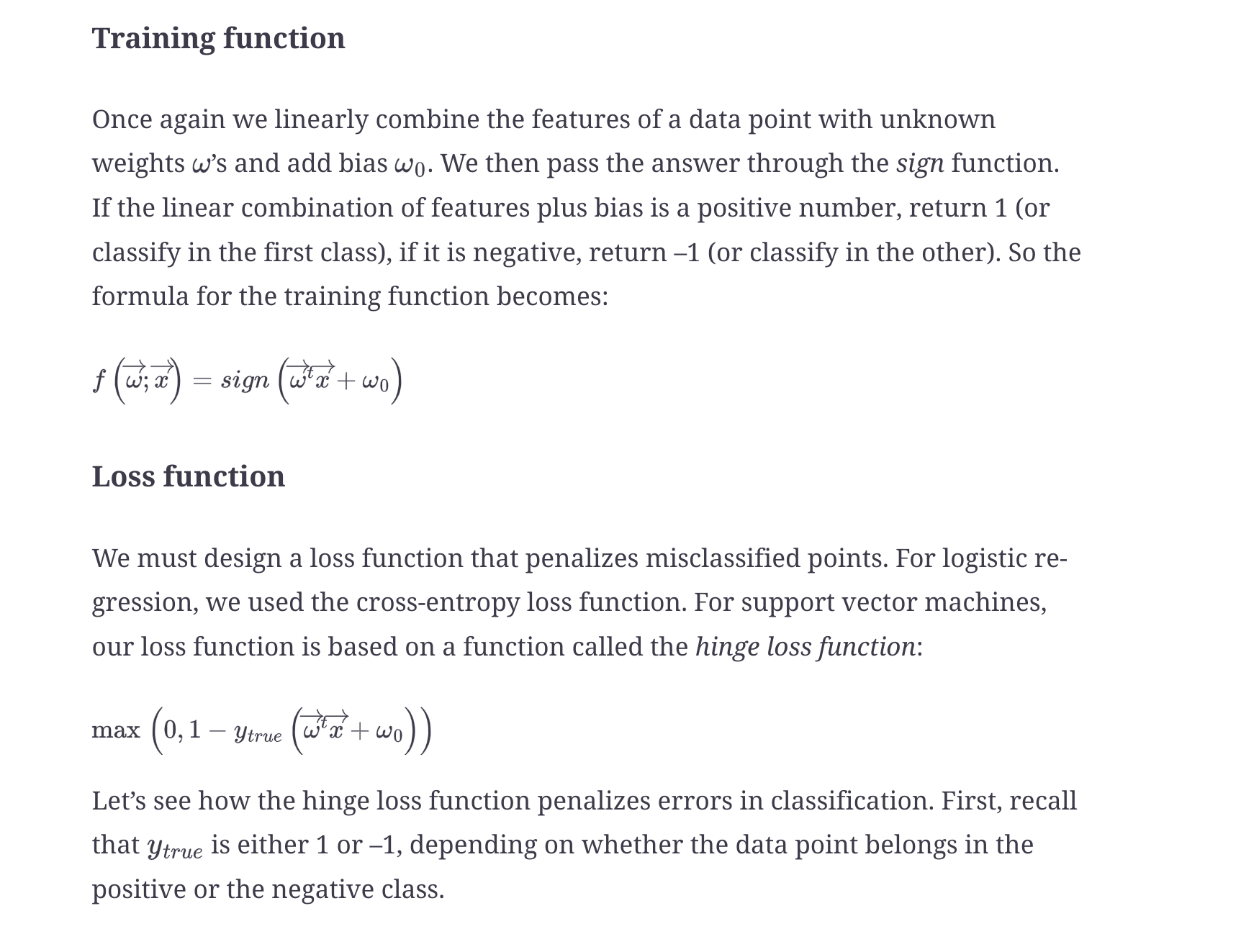
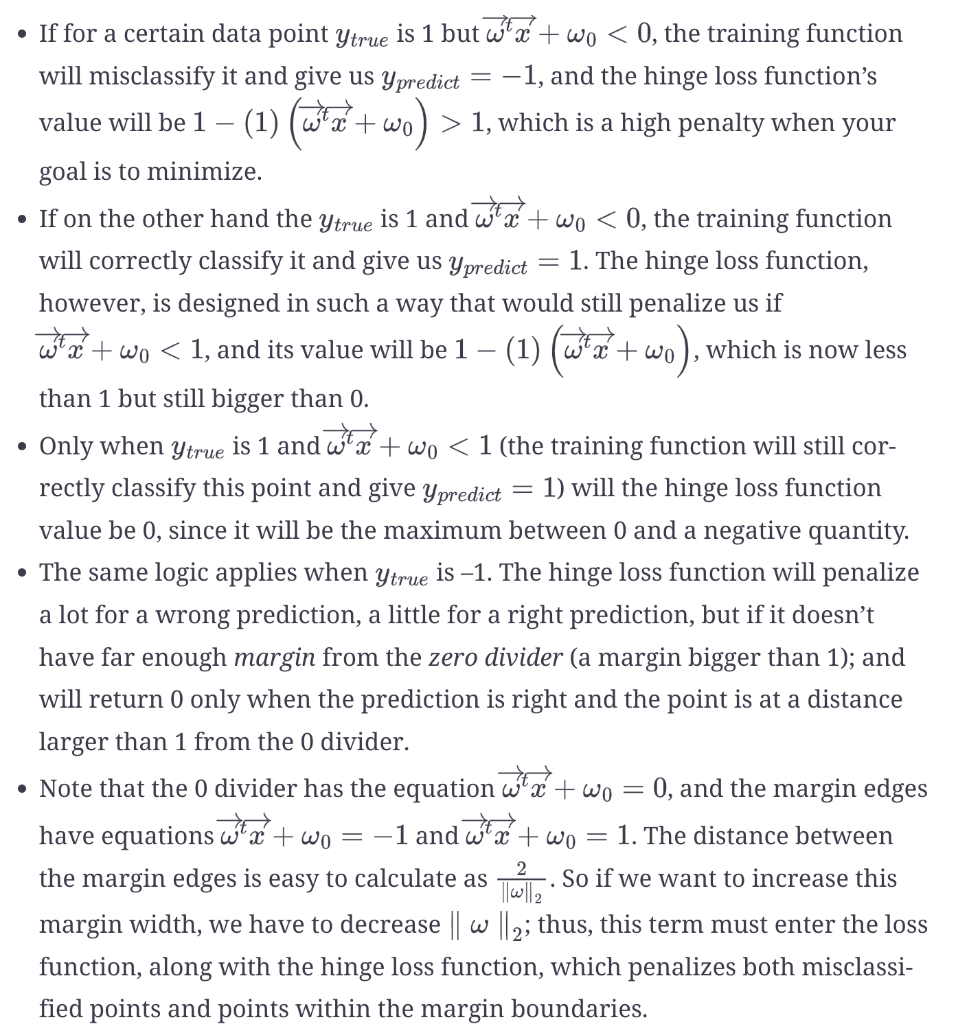
- SVM uses hinge loss function. When the loss is greater than 1 then it is a high penalty, if the loss is between 0 and 1 then it is still penalized and if the loss is 0, there is no penalty.

Decision Tree
- It is a non-parametric model, it does not fix the shape of the function ahead of time.
- This flexibility makes it overfitting to the data
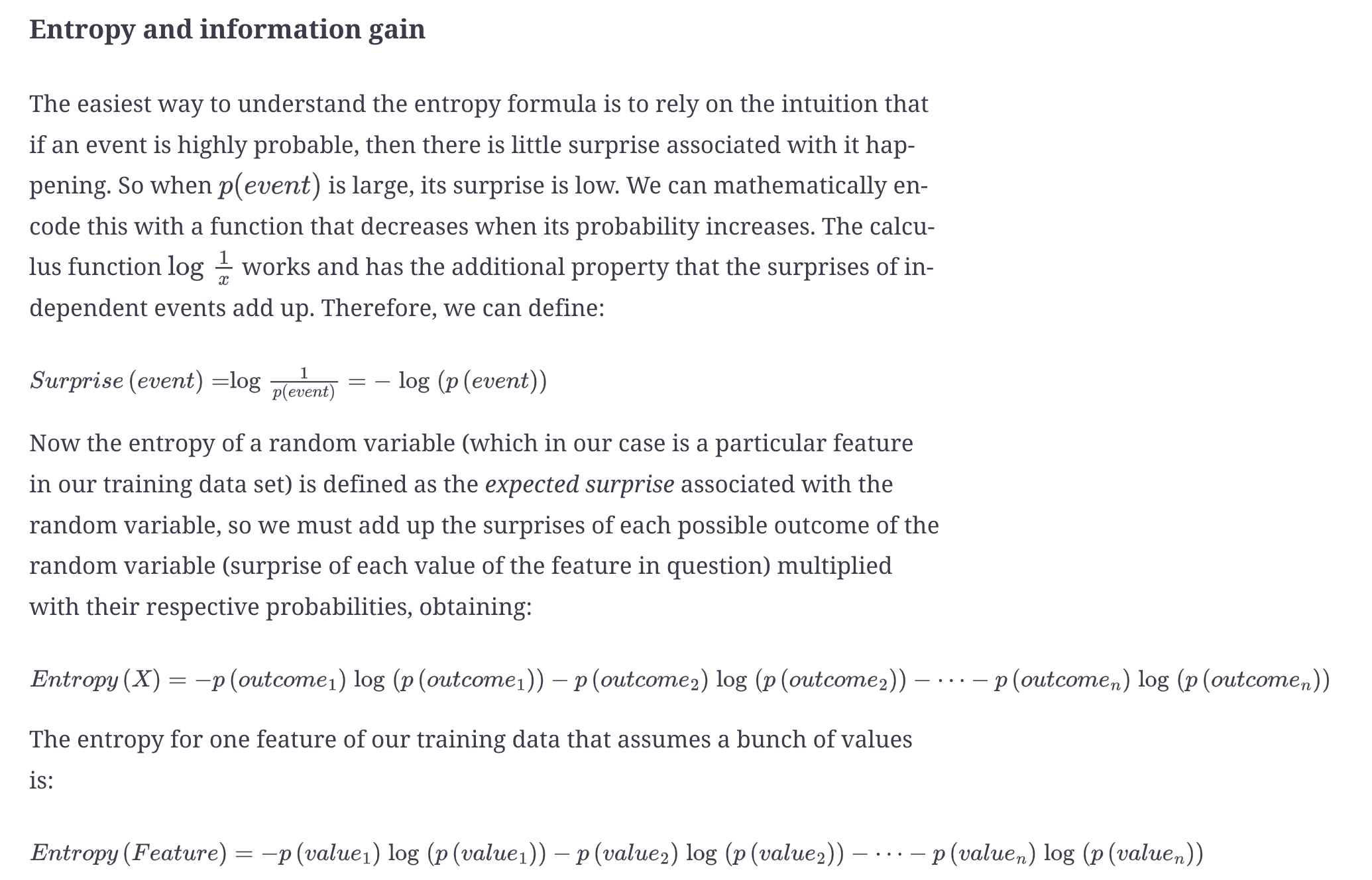
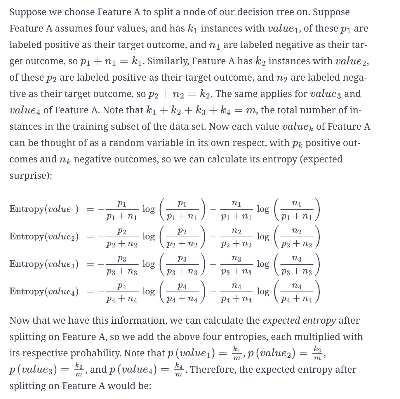
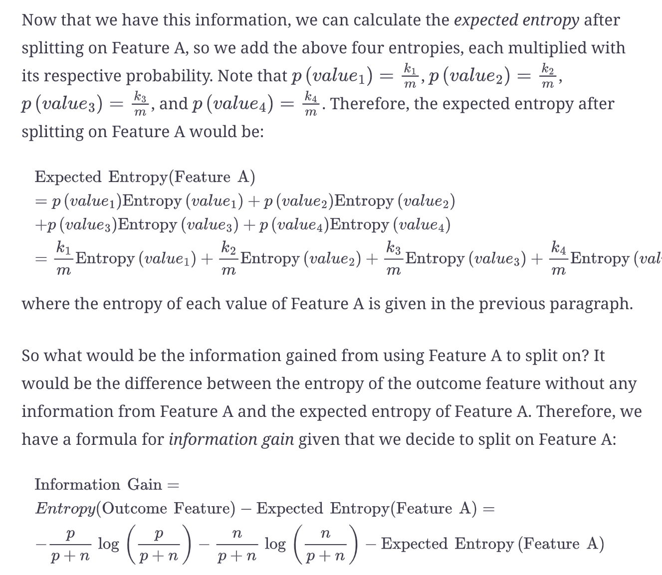
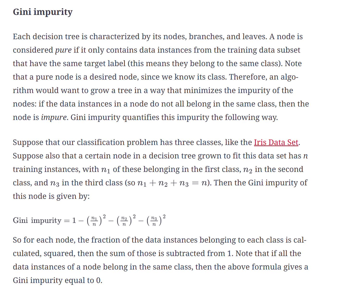
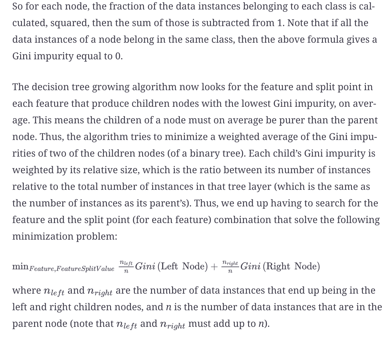
- Entropy and Gini Index are used to measure the importance of a feature. Gini Index is less expensive, so it a default in most packages.
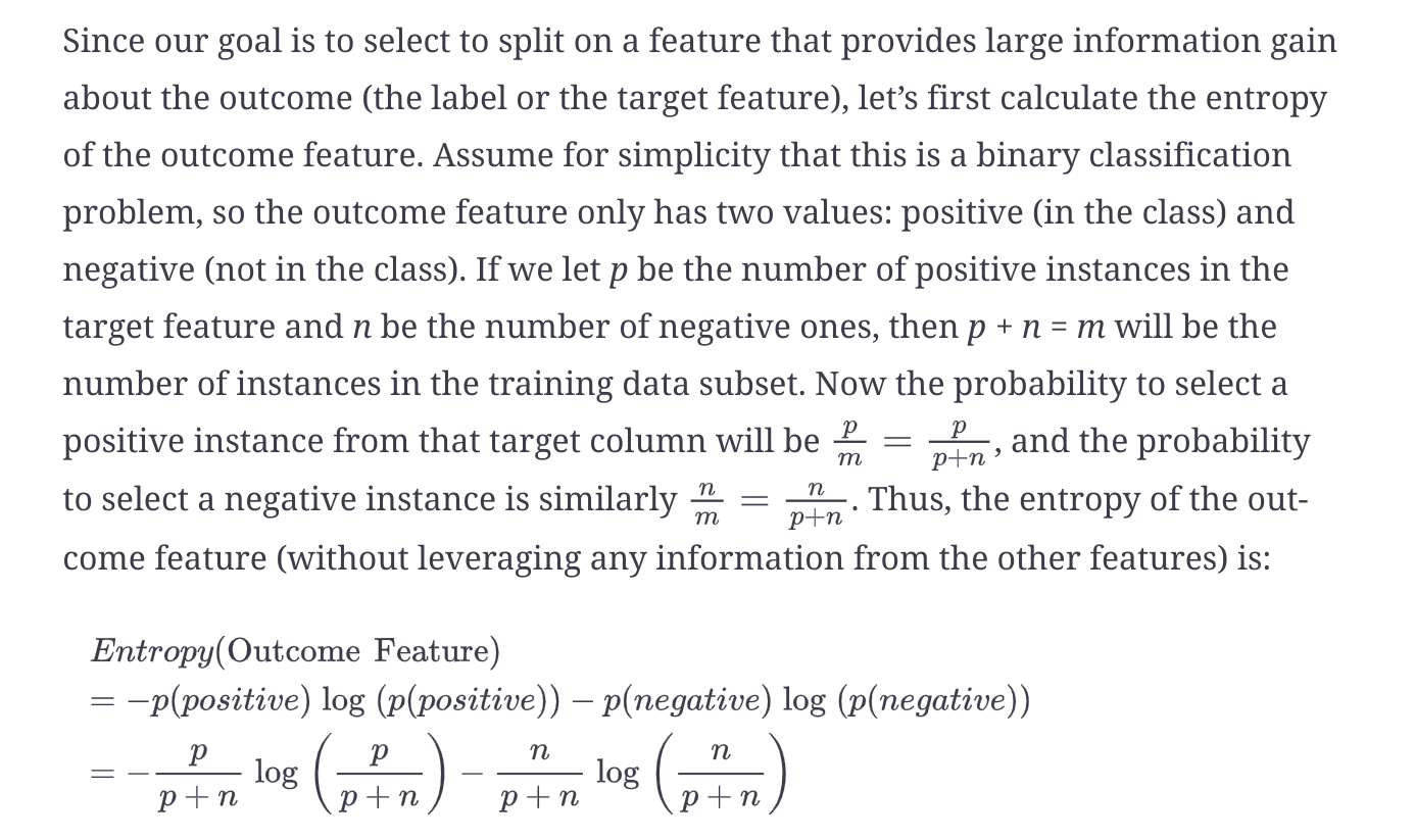
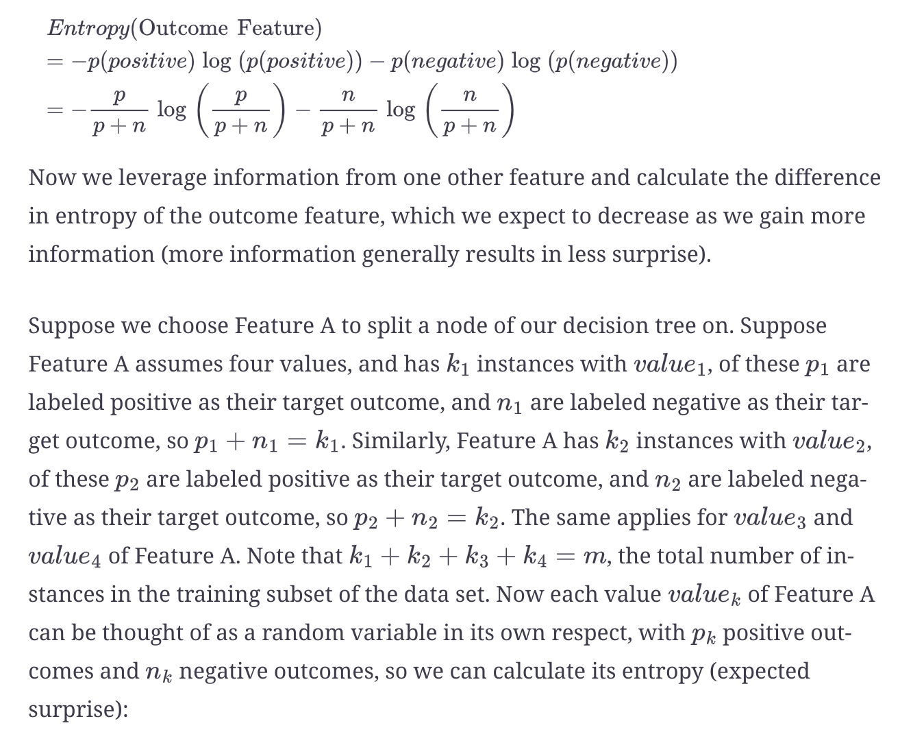
- Entropy approach - Feature split that provides the maximum information gain
- Gini Impurity - Split that provides lowest average Gini Impurity
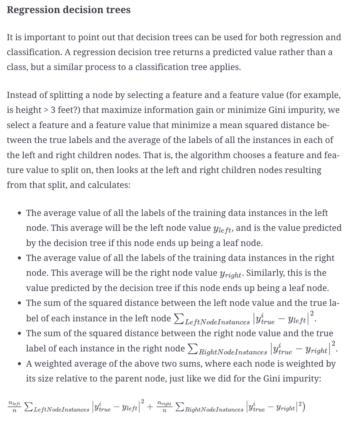
Pros & Cons
- unstable
- Sensitive to rotations in the data, since their decision boundaries are ususally horizontal and vertical. Fix - Transform the data to match its principal axes, using SVD
- overfit the data
K-Means clustering
- It minimizes the variance (the squared euclidean distances to the mean) within each cluster
Feature selection
- F-test and mutual information test for feature selection
What is bagging, pasting, random patches and stacking?
- Bagging is taking random subsets with replacement and pasting taking random subsets without replacement
- Random patches means taking a subset of features for modelling
- Stacking is using a prediction model on all the results of all models to get final prediction
Gradient Descent
Gradient - The effect on the loss by changing a single parameter, while keeping everything else constant. How much the loss changes if one parameter changes a little bit
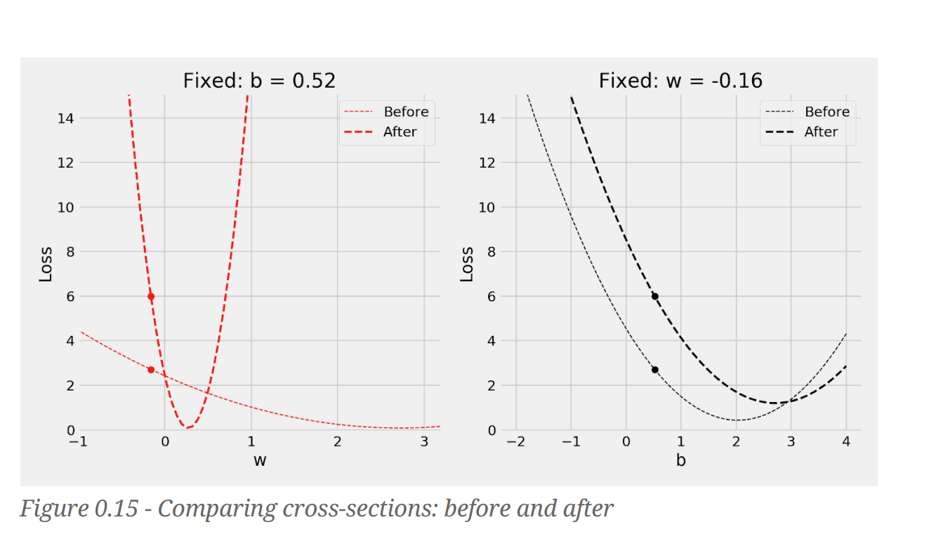
Gradient is steepness. Learning rate can be equated to step size and the steepness dictates the number of steps (relative impact of the parameter). we then take a number of steps that’s proportional to the relative impact: more impact, more steps
As we will be using a single learning rate for all the parameters, the size of the learning rate is limited by the steepest curve. All other curves will be using suboptimal learning rate, given their shapes. (why can’t we use different learning rates for different curves? - Is it a implementation problem or other challenge?)
To make the gradients equally steep - we should do feature standardization or normalization Impact on loss with and without scaling for two parameters. We should use training set only to fit the standardscaler, we should use its transform method to apply the preprocessing step to all datasets: training, validation and test
