Gradient Boosting

• In contrast to Adaboost which uses weights as a surrogate for residuals, gradeint boosting uses these residuals directly!

• Adaboost can be applied loss functions which considers weights for the training data. In contrast gradient boosting is a generalized method widely applicable to many loss functions.

• The framework of gradient boosting can be applied to any loss function, which means that any classification, regression or ranking problem can be “boosted” using weak learners. This flexibility has been a key reason for the emergence and ubiquity of gradient boosting as a state-of-the-art ensemble approach.

Gradient Boosting: Gradient Descent + Boosting

• Like AdaBoost, gradient boosting trains a weak learner to fix the mistakes made by the previous weak learner. Adaboost uses example weights to focus learning on misclassified examples, while gradient boosting uses example residuals to do the same. • Like gradient descent, gradient boosting updates the current model with gradient information. Gradient descent uses the negative gradient directly, while gradient boosting trains a weak regressor over the negative residuals to approximate the gradient.

• 

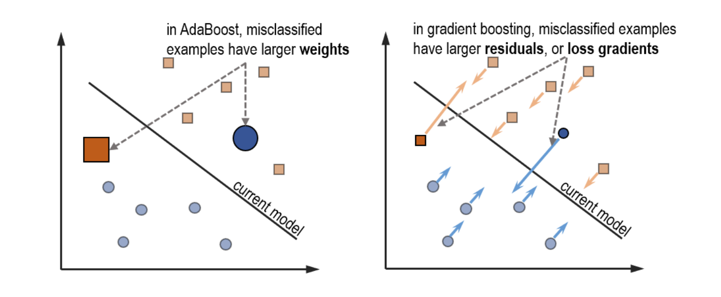
  Adaboost Vs Gradient Boosting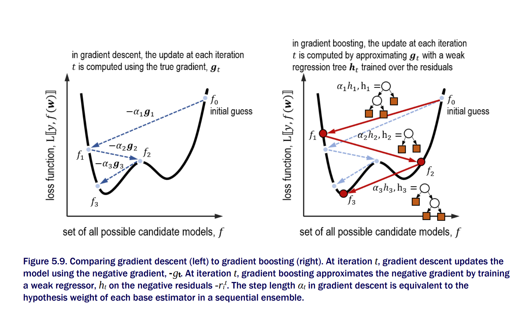

• 

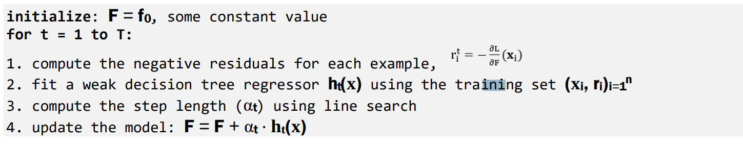
  Gradient Descent for Boosting

• To adapt gradient boosting to a wide variety of loss functions, it adopts two general procedures:-

  • Approximate gradients using weak regressors
  • Compute the model weights using line search

Pseudo code Gradient Boosting

def fit_gradient_boosting (X,y, n_estimators=10):
    n_samples, n_features = X.shape
    n_estimators = 10
    # Initialize an empty ensemble
    estimators = []
    # Predictions of the ensemble on the training set
    F = np.full((n_samples,),0.0)

    for t in range(n_estimators):
        # Compute residuals as negative gradients of the squared loss
        residuals = y - F
        # Fit regression tree to the examples and residuals
        h = DecisionTreeRegressor(max_depth=1)
        h.fit(X,residuals)

        hreg = h.predict(X)
        # Set up the loss function as a line search problem
        loss = lambda a: np.linalg.norm(y - (F + a*hreg))**2
        # Find the best step length using the golden section search
        step = minimize_scalar(loss,method = 'golden')
        a = step.x
        # Update the ensemble predictions
        F += a*hreg
        estimators.append((a,h))

For large datasets, GBM is very slow. For large datasets, the number of splits a tree-learner has to consider becomes prohibitively large

Histogram-based Gradient Boosting

• Trading exactness for speed
• We bin the values of a features to reduce the number of splits considered for evaluating the best split for a node

Gradient Boosting as Gradient Descent

• GBDT (Gradient Boosting Decision Trees) perform gradient descent in functional space. Gradient descent is performed in parameter space.

• In gradient descent we compute the gradient of the loss with respect to the parameters. In gradient boosting, we compute the gradient of the loss with respect to the predictions.

Summary

• Gradient descent is often used to minimize a loss function to train a machine learning model.
• Residuals, or errors between the true labels and model predictions, can be used to characterize correctly classified and poorly classified training examples. This is analogous to how Unlike AdaBoost uses weights.
• Gradient boosting combines gradient descent and boosting to learn a sequential ensemble of weak learners.
• Weak learners in gradient boosting are regression trees that are trained over the residuals of the training examples and approximate the gradient.
• Gradient boosting can be applied to a wide variety of loss functions arising from classification, regression or ranking tasks.
• Histogram-based tree learning trades off exactness for efficiency, allowing us to train gradient boosting models very rapidly and scaling up to larger data sets.
• Learning can be sped up even further by smartly sampling training examples (Gradient OneSide Sampling, GOSS) or smartly bundling features (Exclusive Feature Bundling, EFB).
• LightGBM is a powerful, publicly available framework for gradient boosting that incorporates both GOSS and EFB.
• As with AdaBoost, we can avoid overfitting in gradient boosting by choosing an effective learning rate or via early stopping. LightGBM provides support for both.
• In addition to a wide variety of loss functions for classification, regression and ranking,LightGBM also provides support for incorporation of our own custom, problem-specific loss functions for training.

Explanation from Jeremy Howard

• Additive Modeling - Adding up a bunch of subfunctions to create a composite function that models some data points is called Additive Modeling. GBM use additive modeling to gradually nudge an approximate model towards a reallly good model, by adding simple submodels to a composite model

• The weak model learns direction vectors with direction information, not just magnitudes

• The initial model is trying to learn target y given x, but the weak learners are trying to learn direction vectors given x

• training the weak models on a direction vector that includes the residual magnitude makes the composite model chase outliers. This occurs because mean computations are easily skewed by outliers and our regression tree stumps yield predictions using the mean of the target values in a leaf. For noisy target variables, it makes more sense to focus on the direction of y from the prediction rather than the magnitude and direction.

• While we train the weak models on the sign vector, the weak models are modified to predict a residual not a sign vector!

• Optimizing sign vector leads to a solution that optimized the model according to mean absolute value (MAE) or l1 loss function. (Better than MSE which is sensitive to outliers)

• Optimizing MAE means, we should use median as the prediction for the initial model.

• MSE optimizing GBMs train trees on residual vectors and MAE GBMs train trees on sign vectors

• The second difference between GBMs is that tree leaves of MSE GBMs predict the average of the residuals. MAE GBM tree leaves predict the median of the residual. weak models for both GBMs predict residuals given a feature vector for an observtion.

• Changing the direction vector in a GBM is chasing the negative gradient of a loss function via gradient descent

• Chasing the residual vector in a GBM is chasing the gradient vector of the MSE L2 loss function while performing gradient descent

• Chasing the sign vector in a GBM is chasing the gradient vector of the MAE l1 loss function while performing gradient descent

• `GBM training occurs on two levels, one to train the weak models and one on the overall composite model. It is the overall training of the composite model that performs gradient descent by adding the residual vector (assuming MSE) to get the improved model prediction. Training a NN using gradient descent tweaks model parameters whereas training a GBM tweaks (boost) the model output.

• To summarize, in case of MSE loss, residual is equivalent to the gradient of MSE loss and weight for each leaf is equal to the mean of the residuals in that particular leaf

References:-

• Manning book - Ensemble Methods for ML
• Understanding Gradient Boosting as a gradient descent
• Gradient Boosting code implementation
• Gradient boosting explained by Jeremy Howard
• Gradient Boosting from scratch
• Gradient Boosting Explained