Pivot Table and Grouping in Pandas

import pandas as pd
import numpy as np

Create a dataset

### Create a dataset
import pandas as pd
import numpy as np

# create categorical variables
age_group = pd.Categorical(["18-24", "25-34", "35-44", "45-54", "55-64", "65+", "18-24", "25-34", "35-44", "45-54", "55-64", "65+", "18-24", "25-34", "35-44"])
marital_status = pd.Categorical(["Married", "Single", "Married", "Single", "Widowed", "Divorced", "Married", "Single", "Married", "Single", "Widowed", "Divorced", "Married", "Single", "Married"])
employment_status = pd.Categorical(["Employed", "Unemployed", "Employed", "Unemployed", "Retired", "Employed", "Unemployed", "Employed", "Unemployed", "Employed", "Retired", "Unemployed", "Employed", "Unemployed", "Retired"])
gender = pd.Categorical(["Male", "Female", "Male", "Female", "Male", "Female", "Male", "Female", "Male", "Female", "Male", "Female", "Male", "Female", "Male"])

# create numeric variables
income = np.random.normal(50000, 10000, 15)
education_years = np.random.randint(8, 16, 15)
number_of_children = np.random.randint(0, 5, 15)
hours_worked_per_week = np.random.randint(20, 60, 15)

# create census dataset
census_data = pd.DataFrame({"age_group": age_group, "marital_status": marital_status, "employment_status": employment_status, "gender": gender, "income": income, "education_years": education_years, "number_of_children": number_of_children, "hours_worked_per_week": hours_worked_per_week})
census_data.head(3)

	age_group	marital_status	employment_status	gender	income	education_years	number_of_children	hours_worked_per_week
0	18-24	Married	Employed	Male	54327.605016	12	2	45
1	25-34	Single	Unemployed	Female	51258.164750	14	3	38
2	35-44	Married	Employed	Male	52939.298442	9	2	42

Pivot Table

# what is the average education years for each age_group and employment_status?

(census_data
.pivot_table(index='age_group', columns='employment_status',
    values='education_years', aggfunc='mean')
)

employment_status	Employed	Retired	Unemployed
age_group
18-24	10.5	NaN	12.0
25-34	8.0	NaN	14.5
35-44	9.0	9.0	11.0
45-54	8.0	NaN	15.0
55-64	NaN	14.5	NaN
65+	11.0	NaN	15.0

# Using Max as aggregate function
(census_data
.pivot_table(index='age_group', columns='employment_status',
    values='education_years', aggfunc='max')
)

employment_status	Employed	Retired	Unemployed
age_group
18-24	12.0	NaN	12.0
25-34	8.0	NaN	15.0
35-44	9.0	9.0	11.0
45-54	8.0	NaN	15.0
55-64	NaN	15.0	NaN
65+	11.0	NaN	15.0

Using multiple aggregations

# Find the Min and Max Incomes for all the age groups
(census_data.
    pivot_table(index='age_group', 
         values='income', aggfunc=['min', 'max'])
)

	min	max
	income	income
age_group
18-24	53176.552487	65210.548202
25-34	32718.963301	63933.909067
35-44	52939.298442	66377.414798
45-54	38553.347657	61113.975298
55-64	46070.260269	51285.443271
65+	42717.383692	51510.970139

(census_data.
    pivot_table(index='age_group', 
         values=['income','education_years'], aggfunc=['min', 'max'])
)

	min		max
	education_years	income	education_years	income
age_group
18-24	9	53176.552487	12	65210.548202
25-34	8	32718.963301	15	63933.909067
35-44	9	52939.298442	11	66377.414798
45-54	8	38553.347657	15	61113.975298
55-64	14	46070.260269	15	51285.443271
65+	11	42717.383692	15	51510.970139

Using custom aggregate function in pivot_table

# We can provide a custom aggfunc function to the pivot_table 
# Let us calculate the percentage of people employment for a given age_group
def percentage_of_employment_status(ser):
    return ser.str.contains('Employed').sum() / len(ser) * 100

# We are not provide 'columns' here because we need a single column output
# The custom aggregate function will be applied on the values 'employment_status'
(census_data
.pivot_table(index='age_group', 
    values='employment_status', aggfunc=percentage_of_employment_status)
)

	employment_status
age_group
18-24	66.666667
25-34	33.333333
35-44	33.333333
45-54	50.000000
55-64	0.000000
65+	50.000000

Different Aggregations per column

# For each gender what is the average Income and max hours_worked_per_week
(census_data.
    pivot_table(index='gender',
        aggfunc={'income': 'mean', 'hours_worked_per_week': 'min'})
)

	hours_worked_per_week	income
gender
Female	29	48829.530558
Male	26	55967.094844

Groupby

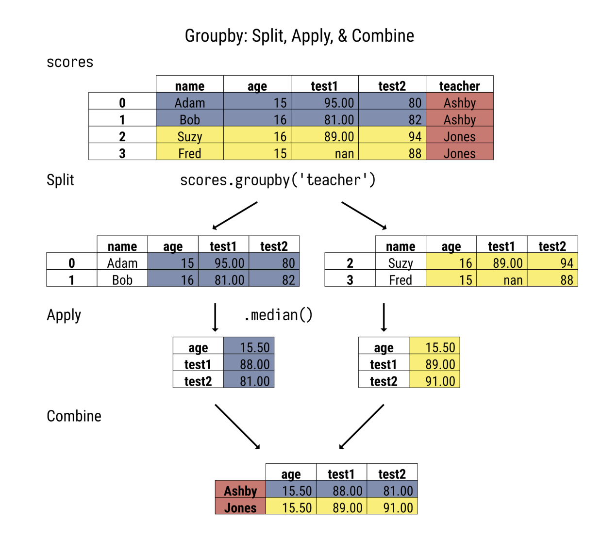
groupby method is lazy and does not perform an aggregation until we specify which aggregation to perform

# This will create a multi-Index series
# The columns in groupby will become the index of the series or dataframe
# we need to unstack the index to get the pivot table
census_data.groupby(['age_group','employment_status'])['education_years'].mean()

age_group  employment_status
18-24      Employed             10.5
           Retired               NaN
           Unemployed           12.0
25-34      Employed              8.0
           Retired               NaN
           Unemployed           14.5
35-44      Employed              9.0
           Retired               9.0
           Unemployed           11.0
45-54      Employed              8.0
           Retired               NaN
           Unemployed           15.0
55-64      Employed              NaN
           Retired              14.5
           Unemployed            NaN
65+        Employed             11.0
           Retired               NaN
           Unemployed           15.0
Name: education_years, dtype: float64

# The below code will unstack the multi-Index and create a pivot table
# The column names are still multi-Index
# We can rename the column names for convineance
census_data.groupby(['age_group','employment_status'])['education_years'].mean().unstack('employment_status')

employment_status	Employed	Retired	Unemployed
age_group
18-24	10.5	NaN	12.0
25-34	8.0	NaN	14.5
35-44	9.0	9.0	11.0
45-54	8.0	NaN	15.0
55-64	NaN	14.5	NaN
65+	11.0	NaN	15.0

# better coding format
(census_data
.groupby(['age_group','employment_status'])
.education_years
.mean()
.unstack('employment_status')
)

employment_status	Employed	Retired	Unemployed
age_group
18-24	10.5	NaN	12.0
25-34	8.0	NaN	14.5
35-44	9.0	9.0	11.0
45-54	8.0	NaN	15.0
55-64	NaN	14.5	NaN
65+	11.0	NaN	15.0

Groupby using custom Aggregate function

(census_data   # dataframe on which to perform groupby
.groupby(['age_group']) # columns to group by
## Pull out the required column on which to perform aggregation
[['employment_status']] # column on which to perform aggregation operation. As we are using '[[' here, the output will be a dataframe. If using '[', the output will be series
.agg(percentage_of_employment_status) # using custom aggregate function
)

	employment_status
age_group
18-24	66.666667
25-34	33.333333
35-44	33.333333
45-54	50.000000
55-64	0.000000
65+	50.000000

groupby aggregation on multiple columns

# Find the Min and Max Incomes for all the age groups
(census_data.
    groupby(['age_group'])
    [['income', 'education_years']]
    .agg(['min', 'max'])
)

	income		education_years
	min	max	min	max
age_group
18-24	53176.552487	65210.548202	9	12
25-34	32718.963301	63933.909067	8	15
35-44	52939.298442	66377.414798	9	11
45-54	38553.347657	61113.975298	8	15
55-64	46070.260269	51285.443271	14	15
65+	42717.383692	51510.970139	11	15

Different aggregations per column

# For each gender what is the average Income and max hours_worked_per_week
(census_data
    .groupby('gender')
    .agg({'income': ['min','max','mean'], 'hours_worked_per_week': 'min'})
)

	income			hours_worked_per_week
	min	max	mean	min
gender
Female	32718.963301	63933.909067	48829.530558	29
Male	46070.260269	66377.414798	55967.094844	26

Named Aggregations

We can use this functionality to name the columns when using groupby
We can use keyword parameter in agg function, which will turn into a column name
The input for keyword parameter will be a tuple - (column_name, agg_function)
Use Named Aggregations for flat column names
When performing groupby with multiple categorical columns, pandas will create the cartesian product of those columns even if there is no corresponding value.
This is not available for pivot_table

(census_data
.groupby('gender')
.agg(min_income=('income','min'),
    max_income=('income','max'),
    mean_income=('income','mean'),
    min_hours_worked_per_week=('hours_worked_per_week','min'),
    max_hours_worked_per_week=('hours_worked_per_week','max')
    )
)

	min_income	max_income	mean_income	min_hours_worked_per_week	max_hours_worked_per_week
gender
Female	32718.963301	63933.909067	48829.530558	29	54
Male	46070.260269	66377.414798	55967.094844	26	59

Grouping with Functions

def even_grouper(idx):
    return 'odd' if idx % 2  else 'even'

census_data.pivot_table(index=even_grouper, aggfunc='size')

even    8
odd     7
dtype: int64

(census_data
.groupby(even_grouper)
.size()
)

even    8
odd     7
dtype: int64

Stacking and Unstacking

Unstack moves an index into the columns
We use this on multi-index data, moving one of the indices into the columns
stack method does the reverse, moving multi-level column into the index

(census_data
.groupby(['age_group','employment_status'])
.size()
)

age_group  employment_status
18-24      Employed             2
           Retired              0
           Unemployed           1
25-34      Employed             1
           Retired              0
           Unemployed           2
35-44      Employed             1
           Retired              1
           Unemployed           1
45-54      Employed             1
           Retired              0
           Unemployed           1
55-64      Employed             0
           Retired              2
           Unemployed           0
65+        Employed             1
           Retired              0
           Unemployed           1
dtype: int64

# Unstacking a series into a dataframe
(census_data
.groupby(['age_group','employment_status'])
.size()
.unstack('employment_status'))

employment_status	Employed	Retired	Unemployed
age_group
18-24	2	0	1
25-34	1	0	2
35-44	1	1	1
45-54	1	0	1
55-64	0	2	0
65+	1	0	1

# Unstacking a index of a dataframe into nested columns
(census_data
.groupby(['age_group','employment_status'])
.mean(numeric_only=True)
.unstack('employment_status'))

	income			education_years			number_of_children			hours_worked_per_week
employment_status	Employed	Retired	Unemployed	Employed	Retired	Unemployed	Employed	Retired	Unemployed	Employed	Retired	Unemployed
age_group
18-24	53752.078752	NaN	65210.548202	10.5	NaN	12.0	1.0	NaN	4.0	35.5	NaN	36.0
25-34	63933.909067	NaN	41988.564026	8.0	NaN	14.5	4.0	NaN	1.5	33.0	NaN	46.0
35-44	52939.298442	58349.636265	66377.414798	9.0	9.0	11.0	2.0	1.0	2.0	42.0	51.0	51.0
45-54	61113.975298	NaN	38553.347657	8.0	NaN	15.0	0.0	NaN	0.0	34.0	NaN	29.0
55-64	NaN	48677.851770	NaN	NaN	14.5	NaN	NaN	2.5	NaN	NaN	55.5	NaN
65+	42717.383692	NaN	51510.970139	11.0	NaN	15.0	0.0	NaN	4.0	53.0	NaN	35.0

# Stacking
# We take nested columns and send it to index
# This is the opposite of stacking
# The outermost column is 0 and the inner columns are 1
(census_data.
    pivot_table(index='age_group', 
          aggfunc={'income':['min','max'], 'hours_worked_per_week':['min','max']})
)

	hours_worked_per_week		income
	max	min	max	min
age_group
18-24	45	26	65210.548202	53176.552487
25-34	54	33	63933.909067	32718.963301
35-44	51	42	66377.414798	52939.298442
45-54	34	29	61113.975298	38553.347657
55-64	59	52	51285.443271	46070.260269
65+	53	35	51510.970139	42717.383692

# Stacking the outer column
(census_data.
    pivot_table(index='age_group', 
          aggfunc={'income':['min','max'], 'hours_worked_per_week':['min','max']})
    .stack(0)
)

		max	min
age_group
18-24	hours_worked_per_week	45.000000	26.000000
18-24	income	65210.548202	53176.552487
25-34	hours_worked_per_week	54.000000	33.000000
25-34	income	63933.909067	32718.963301
35-44	hours_worked_per_week	51.000000	42.000000
35-44	income	66377.414798	52939.298442
45-54	hours_worked_per_week	34.000000	29.000000
45-54	income	61113.975298	38553.347657
55-64	hours_worked_per_week	59.000000	52.000000
55-64	income	51285.443271	46070.260269
65+	hours_worked_per_week	53.000000	35.000000
65+	income	51510.970139	42717.383692

# Stacking the inner column
(census_data.
    pivot_table(index='age_group', 
          aggfunc={'income':['min','max'], 'hours_worked_per_week':['min','max']})
    .stack(1)
)

		hours_worked_per_week	income
age_group
18-24	max	45	65210.548202
18-24	min	26	53176.552487
25-34	max	54	63933.909067
25-34	min	33	32718.963301
35-44	max	51	66377.414798
35-44	min	42	52939.298442
45-54	max	34	61113.975298
45-54	min	29	38553.347657
55-64	max	59	51285.443271
55-64	min	52	46070.260269
65+	max	53	51510.970139
65+	min	35	42717.383692

Flatenning the Hierarchial Index

# We can use 'reset_index' method to make the indexes columns of a df
(census_data
.groupby(['age_group','employment_status'])
['income']
.mean()
)

age_group  employment_status
18-24      Employed             53752.078752
           Retired                       NaN
           Unemployed           65210.548202
25-34      Employed             63933.909067
           Retired                       NaN
           Unemployed           41988.564026
35-44      Employed             52939.298442
           Retired              58349.636265
           Unemployed           66377.414798
45-54      Employed             61113.975298
           Retired                       NaN
           Unemployed           38553.347657
55-64      Employed                      NaN
           Retired              48677.851770
           Unemployed                    NaN
65+        Employed             42717.383692
           Retired                       NaN
           Unemployed           51510.970139
Name: income, dtype: float64

# Using reset_index will make the index columns and flatten the hierarchy
(census_data
.groupby(['age_group','employment_status'])
['income']
.mean()
.reset_index()
)

	age_group	employment_status	income
0	18-24	Employed	53752.078752
1	18-24	Retired	NaN
2	18-24	Unemployed	65210.548202
3	25-34	Employed	63933.909067
4	25-34	Retired	NaN
5	25-34	Unemployed	41988.564026
6	35-44	Employed	52939.298442
7	35-44	Retired	58349.636265
8	35-44	Unemployed	66377.414798
9	45-54	Employed	61113.975298
10	45-54	Retired	NaN
11	45-54	Unemployed	38553.347657
12	55-64	Employed	NaN
13	55-64	Retired	48677.851770
14	55-64	Unemployed	NaN
15	65+	Employed	42717.383692
16	65+	Retired	NaN
17	65+	Unemployed	51510.970139

Flattening the hierarchial columns

def flatten_cols(df):
    cols = ['_'.join(map(str, vals)) for vals in df.columns.to_flat_index()]
    df.columns = cols
    return df

(census_data
.pivot_table(index='age_group', 
          aggfunc={'income':['min','max'], 'hours_worked_per_week':['min','max']})
.pipe(flatten_cols)    
)

	hours_worked_per_week_max	hours_worked_per_week_min	income_max	income_min
age_group
18-24	45	26	65210.548202	53176.552487
25-34	54	33	63933.909067	32718.963301
35-44	51	42	66377.414798	52939.298442
45-54	34	29	61113.975298	38553.347657
55-64	59	52	51285.443271	46070.260269
65+	53	35	51510.970139	42717.383692