Telecom Churn Prediction

The objectives of this project are:-
1. Perform exploratory analysis and extract insights from the dataset.
2. Split the dataset into train/test sets and explain your reasoning.
3. Build a predictive model to predict which customers are going to churn and discuss the reason why you choose a particular algorithm.
4. Establish metrics to evaluate model performance.
5. Discuss the potential issues with deploying the model into production

Import the required libraries

# python version # 3.8.2
import pandas as pd 
import numpy as np 
from pandas_profiling import ProfileReport 
from pycaret.classification import * 
from sklearn import metrics 
import os 
from sklearn.model_selection import train_test_split 

import warnings
warnings.filterwarnings('ignore')

# option to display all columns
pd.set_option('display.max_columns', None)

# Read the data
telecom_churn = pd.read_csv('data science challenge.csv')

telecom_churn.head(10)

	state	account length	area code	phone number	international plan	voice mail plan	number vmail messages	total day minutes	total day calls	total day charge	total eve minutes	total eve calls	total eve charge	total night minutes	total night calls	total night charge	total intl minutes	total intl calls	total intl charge	customer service calls	churn
0	KS	128	415	382-4657	no	yes	25	265.1	110	45.07	197.4	99	16.78	244.7	91	11.01	10.0	3	2.70	1	False
1	OH	107	415	371-7191	no	yes	26	161.6	123	27.47	195.5	103	16.62	254.4	103	11.45	13.7	3	3.70	1	False
2	NJ	137	415	358-1921	no	no	0	243.4	114	41.38	121.2	110	10.30	162.6	104	7.32	12.2	5	3.29	0	False
3	OH	84	408	375-9999	yes	no	0	299.4	71	50.90	61.9	88	5.26	196.9	89	8.86	6.6	7	1.78	2	False
4	OK	75	415	330-6626	yes	no	0	166.7	113	28.34	148.3	122	12.61	186.9	121	8.41	10.1	3	2.73	3	False
5	AL	118	510	391-8027	yes	no	0	223.4	98	37.98	220.6	101	18.75	203.9	118	9.18	6.3	6	1.70	0	False
6	MA	121	510	355-9993	no	yes	24	218.2	88	37.09	348.5	108	29.62	212.6	118	9.57	7.5	7	2.03	3	False
7	MO	147	415	329-9001	yes	no	0	157.0	79	26.69	103.1	94	8.76	211.8	96	9.53	7.1	6	1.92	0	False
8	LA	117	408	335-4719	no	no	0	184.5	97	31.37	351.6	80	29.89	215.8	90	9.71	8.7	4	2.35	1	False
9	WV	141	415	330-8173	yes	yes	37	258.6	84	43.96	222.0	111	18.87	326.4	97	14.69	11.2	5	3.02	0	False

Check the Shape and Column types of the Dataframe

telecom_churn.shape

(3333, 21)

telecom_churn.dtypes

state                      object
account length              int64
area code                   int64
phone number               object
international plan         object
voice mail plan            object
number vmail messages       int64
total day minutes         float64
total day calls             int64
total day charge          float64
total eve minutes         float64
total eve calls             int64
total eve charge          float64
total night minutes       float64
total night calls           int64
total night charge        float64
total intl minutes        float64
total intl calls            int64
total intl charge         float64
customer service calls      int64
churn                        bool
dtype: object

Exploratory Analysis

# No missing values in the data.
# Scaling of numeric columns is required
telecom_churn.describe()

	account length	area code	number vmail messages	total day minutes	total day calls	total day charge	total eve minutes	total eve calls	total eve charge	total night minutes	total night calls	total night charge	total intl minutes	total intl calls	total intl charge	customer service calls
count	3333.000000	3333.000000	3333.000000	3333.000000	3333.000000	3333.000000	3333.000000	3333.000000	3333.000000	3333.000000	3333.000000	3333.000000	3333.000000	3333.000000	3333.000000	3333.000000
mean	101.064806	437.182418	8.099010	179.775098	100.435644	30.562307	200.980348	100.114311	17.083540	200.872037	100.107711	9.039325	10.237294	4.479448	2.764581	1.562856
std	39.822106	42.371290	13.688365	54.467389	20.069084	9.259435	50.713844	19.922625	4.310668	50.573847	19.568609	2.275873	2.791840	2.461214	0.753773	1.315491
min	1.000000	408.000000	0.000000	0.000000	0.000000	0.000000	0.000000	0.000000	0.000000	23.200000	33.000000	1.040000	0.000000	0.000000	0.000000	0.000000
25%	74.000000	408.000000	0.000000	143.700000	87.000000	24.430000	166.600000	87.000000	14.160000	167.000000	87.000000	7.520000	8.500000	3.000000	2.300000	1.000000
50%	101.000000	415.000000	0.000000	179.400000	101.000000	30.500000	201.400000	100.000000	17.120000	201.200000	100.000000	9.050000	10.300000	4.000000	2.780000	1.000000
75%	127.000000	510.000000	20.000000	216.400000	114.000000	36.790000	235.300000	114.000000	20.000000	235.300000	113.000000	10.590000	12.100000	6.000000	3.270000	2.000000
max	243.000000	510.000000	51.000000	350.800000	165.000000	59.640000	363.700000	170.000000	30.910000	395.000000	175.000000	17.770000	20.000000	20.000000	5.400000	9.000000

# Format the column names, remove space and special characters in column names
telecom_churn.columns =  telecom_churn.columns.str.strip().str.lower().str.replace(' ', '_').str.replace('(', '').str.replace(')', '')

telecom_churn

	state	account_length	area_code	phone_number	international_plan	voice_mail_plan	number_vmail_messages	total_day_minutes	total_day_calls	total_day_charge	total_eve_minutes	total_eve_calls	total_eve_charge	total_night_minutes	total_night_calls	total_night_charge	total_intl_minutes	total_intl_calls	total_intl_charge	customer_service_calls	churn
0	KS	128	415	382-4657	no	yes	25	265.1	110	45.07	197.4	99	16.78	244.7	91	11.01	10.0	3	2.70	1	False
1	OH	107	415	371-7191	no	yes	26	161.6	123	27.47	195.5	103	16.62	254.4	103	11.45	13.7	3	3.70	1	False
2	NJ	137	415	358-1921	no	no	0	243.4	114	41.38	121.2	110	10.30	162.6	104	7.32	12.2	5	3.29	0	False
3	OH	84	408	375-9999	yes	no	0	299.4	71	50.90	61.9	88	5.26	196.9	89	8.86	6.6	7	1.78	2	False
4	OK	75	415	330-6626	yes	no	0	166.7	113	28.34	148.3	122	12.61	186.9	121	8.41	10.1	3	2.73	3	False
...	...	...	...	...	...	...	...	...	...	...	...	...	...	...	...	...	...	...	...	...	...
3328	AZ	192	415	414-4276	no	yes	36	156.2	77	26.55	215.5	126	18.32	279.1	83	12.56	9.9	6	2.67	2	False
3329	WV	68	415	370-3271	no	no	0	231.1	57	39.29	153.4	55	13.04	191.3	123	8.61	9.6	4	2.59	3	False
3330	RI	28	510	328-8230	no	no	0	180.8	109	30.74	288.8	58	24.55	191.9	91	8.64	14.1	6	3.81	2	False
3331	CT	184	510	364-6381	yes	no	0	213.8	105	36.35	159.6	84	13.57	139.2	137	6.26	5.0	10	1.35	2	False
3332	TN	74	415	400-4344	no	yes	25	234.4	113	39.85	265.9	82	22.60	241.4	77	10.86	13.7	4	3.70	0	False

3333 rows × 21 columns

#telecom_churn["area_code"] = telecom_churn["area_code"].astype('category')

profile = ProfileReport(telecom_churn, title = "Telecom Churn Report")

# create report for EDA
profile.to_widgets()

#save the profile report
profile.to_file("telecom_churn_eda.html")

[telecom_churn.churn.value_counts()]

[False    2850
 True      483
 Name: churn, dtype: int64]

pd.crosstab(telecom_churn.churn, telecom_churn. customer_service_calls,margins=True, margins_name="Total")

customer_service_calls	0	1	2	3	4	5	6	7	8	9	Total
churn
False	605	1059	672	385	90	26	8	4	1	0	2850
True	92	122	87	44	76	40	14	5	1	2	483
Total	697	1181	759	429	166	66	22	9	2	2	3333

import matplotlib.pyplot as plt
ct = pd.crosstab(telecom_churn.churn, telecom_churn.customer_service_calls)
ct.plot.bar(stacked=True)
plt.legend(title='churn vs Number of calls')
plt.show()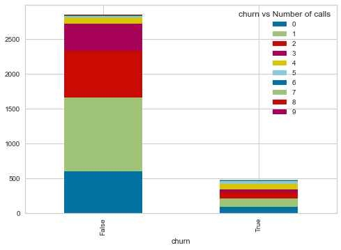

telecom_churn['area_code'].value_counts().plot.bar()

<AxesSubplot:>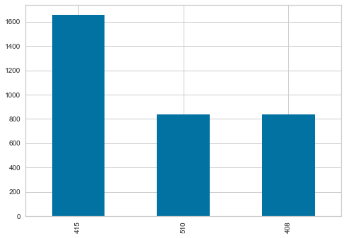

telecom_churn['state'].value_counts().head(10).plot.bar()

<AxesSubplot:>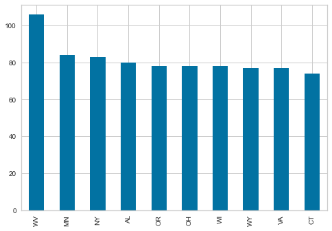

telecom_churn['international_plan'].value_counts().plot.bar()

<AxesSubplot:>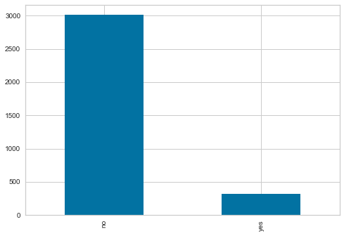

telecom_churn['voice_mail_plan'].value_counts().plot.bar()

<AxesSubplot:>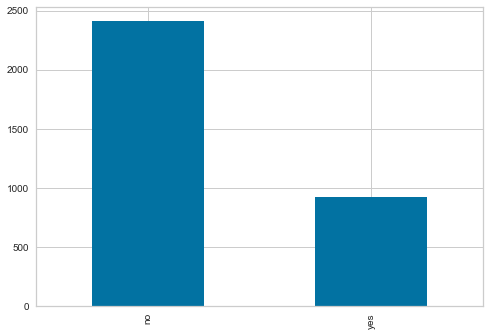

Observations from EDA are:-

1. Dataset is imbalanced - 85.5% customers did not churn and 14.5% customers churned
2. State consist of 51 distinct values with high cardinality
3. Numeric variables are in different ranges and needs to be scaled
4. Three distinct area codes - Area code ‘415’ is 49.7%, rest two area codes are equally distributed
5. Distinct values of phone number is equal to the length of the dataset. This will be equivalent to primary key of the dataset. Not be included in modelling
6. 72.3% customers did not activate their voicemail plan. This is verified by equal number of customers with zero number of voice messages
7. Total international calls and customer service calls data is skewed. This is verified by high kurtosis and skewness.
8. All the other numeric variables are following normal distribution as verified by kurtosis / skewness values and histogram

Split the Data for Training and Testing

The Machine learning algorithm should not be exposed to test data. The performance of the learning algorithm can only be measured by testing on unseen data. To achieve the same a train and test split with 95% and 5% is created. It is ensured that the sampling is stratified so that the proportion of churn and not churn customers are equal in train and test data. As the amount of data is very less, only 5% of the data is kept aside for testing.Further the train data is further split into train and validation set with 90% and 10%. Validation set is required for hyperparameter tuning.As validation set is also exposed to training algorithm, it is also should not be used for model validation. Model validation is done on test set only.

# convert the target value to integers. 
telecom_churn['churn'] = telecom_churn['churn'] * 1

train, test = train_test_split(telecom_churn, test_size = 0.05, stratify = telecom_churn['churn']) 
print('Data for Modeling: ' + str(train.shape))
print('Unseen Data For Predictions: ' + str(test.shape))

Data for Modeling: (3166, 21)
Unseen Data For Predictions: (167, 21)

# Test the proportion of churn in train and test sets
train.churn.value_counts()

0    2707
1     459
Name: churn, dtype: int64

# 16.5% of the customers churned in train data
(459/2707)*100

16.956039896564462

test.churn.value_counts()

0    143
1     24
Name: churn, dtype: int64

# 16.7% of the customers churned in test data
(24/143)*100
# customers churned proportionally from train and test data

16.783216783216783

Modelling with Pycaret

1. Train and validation sets are created with 90 % and 10 % data.
2. The random seed selected for the modeling is 786
3. In this step we are normalizing the data, ignoring the variable ‘phone number’ for analysis
4. Fixing the imbalance in the data using SMOTE method
5. We are transforming the features - Changing the distribution of variables to a normal or approximate normal distribution
6. Ignorning features with low variance - This will ignore variables (multi level categorical) where a single level dominates and there is not much variation in the information provided by the feature
7. The setup is inferring the customer_service_calls as numeric (as there are only ten distinct values). Hence explicitly mentioning it as numeric

exp_clf =    setup(data = train, target = 'churn', session_id = 786, 
                   train_size = 0.9,
                   normalize = True,
                   transformation = True,
                   ignore_low_variance = True,               
                   ignore_features = ['phone_number'],
                   fix_imbalance = True,
                   high_cardinality_features = ['state'],
                   numeric_features = ['customer_service_calls'])               

Setup Succesfully Completed!

	Description	Value
0	session_id	786
1	Target Type	Binary
2	Label Encoded	None
3	Original Data	(3166, 21)
4	Missing Values	False
5	Numeric Features	15
6	Categorical Features	5
7	Ordinal Features	False
8	High Cardinality Features	True
9	High Cardinality Method	frequency
10	Sampled Data	(3166, 21)
11	Transformed Train Set	(2849, 22)
12	Transformed Test Set	(317, 22)
13	Numeric Imputer	mean
14	Categorical Imputer	constant
15	Normalize	True
16	Normalize Method	zscore
17	Transformation	True
18	Transformation Method	yeo-johnson
19	PCA	False
20	PCA Method	None
21	PCA Components	None
22	Ignore Low Variance	True
23	Combine Rare Levels	False
24	Rare Level Threshold	None
25	Numeric Binning	False
26	Remove Outliers	False
27	Outliers Threshold	None
28	Remove Multicollinearity	False
29	Multicollinearity Threshold	None
30	Clustering	False
31	Clustering Iteration	None
32	Polynomial Features	False
33	Polynomial Degree	None
34	Trignometry Features	False
35	Polynomial Threshold	None
36	Group Features	False
37	Feature Selection	False
38	Features Selection Threshold	None
39	Feature Interaction	False
40	Feature Ratio	False
41	Interaction Threshold	None
42	Fix Imbalance	True
43	Fix Imbalance Method	SMOTE

compare_models(fold = 5)

	Model	Accuracy	AUC	Recall	Prec.	F1	Kappa	MCC	TT (Sec)
0	Light Gradient Boosting Machine	0.9512	0.9127	0.7771	0.8732	0.8213	0.7932	0.7957	0.1908
1	Extreme Gradient Boosting	0.9488	0.9145	0.7675	0.8652	0.8124	0.7829	0.7854	0.2130
2	CatBoost Classifier	0.9466	0.9140	0.7577	0.8583	0.8041	0.7734	0.7759	4.3314
3	Extra Trees Classifier	0.9333	0.9032	0.6535	0.8544	0.7392	0.7018	0.7109	0.1456
4	Random Forest Classifier	0.9330	0.9082	0.7045	0.8147	0.7529	0.7145	0.7186	0.0366
5	Gradient Boosting Classifier	0.9308	0.9078	0.7674	0.7618	0.7635	0.7230	0.7238	1.1674
6	Decision Tree Classifier	0.8929	0.8227	0.7238	0.6106	0.6616	0.5986	0.6022	0.0356
7	Ada Boost Classifier	0.8645	0.8464	0.6003	0.5325	0.5625	0.4829	0.4853	0.2996
8	Naive Bayes	0.8284	0.7894	0.6439	0.4430	0.5233	0.4237	0.4355	0.0028
9	K Neighbors Classifier	0.7715	0.7897	0.6878	0.3531	0.4664	0.3398	0.3705	0.0160
10	Logistic Regression	0.7375	0.7886	0.6852	0.3152	0.4314	0.2904	0.3273	0.0316
11	Ridge Classifier	0.7371	0.0000	0.6852	0.3149	0.4311	0.2899	0.3270	0.0082
12	Linear Discriminant Analysis	0.7336	0.7844	0.6779	0.3103	0.4252	0.2824	0.3190	0.0144
13	SVM - Linear Kernel	0.7329	0.0000	0.6079	0.3163	0.4021	0.2621	0.2910	0.0198
14	Quadratic Discriminant Analysis	0.5907	0.6505	0.6373	0.2089	0.3106	0.1201	0.1596	0.0110

LGBMClassifier(boosting_type='gbdt', class_weight=None, colsample_bytree=1.0,
               importance_type='split', learning_rate=0.1, max_depth=-1,
               min_child_samples=20, min_child_weight=0.001, min_split_gain=0.0,
               n_estimators=100, n_jobs=-1, num_leaves=31, objective=None,
               random_state=786, reg_alpha=0.0, reg_lambda=0.0, silent=True,
               subsample=1.0, subsample_for_bin=200000, subsample_freq=0)

Creating the models for top performing algorithms based on Precision and AUC. Tree based models are performing well on this dataset

lightgbm = create_model('lightgbm', fold =5)

	Accuracy	AUC	Recall	Prec.	F1	Kappa	MCC
0	0.9526	0.9008	0.8171	0.8481	0.8323	0.8047	0.8049
1	0.9561	0.9271	0.8193	0.8718	0.8447	0.8192	0.8197
2	0.9544	0.9241	0.8072	0.8701	0.8375	0.8110	0.8118
3	0.9544	0.9278	0.7470	0.9254	0.8267	0.8007	0.8068
4	0.9385	0.8836	0.6951	0.8507	0.7651	0.7301	0.7351
Mean	0.9512	0.9127	0.7771	0.8732	0.8213	0.7932	0.7957
SD	0.0065	0.0176	0.0488	0.0278	0.0287	0.0321	0.0307

catboost = create_model('catboost', fold =5)

	Accuracy	AUC	Recall	Prec.	F1	Kappa	MCC
0	0.9421	0.9161	0.7439	0.8356	0.7871	0.7537	0.7554
1	0.9456	0.9254	0.7711	0.8421	0.8050	0.7735	0.7745
2	0.9561	0.9198	0.8313	0.8625	0.8466	0.8210	0.8212
3	0.9544	0.9314	0.7470	0.9254	0.8267	0.8007	0.8068
4	0.9350	0.8775	0.6951	0.8261	0.7550	0.7178	0.7214
Mean	0.9466	0.9140	0.7577	0.8583	0.8041	0.7734	0.7759
SD	0.0078	0.0190	0.0443	0.0356	0.0317	0.0360	0.0358

xgboost = create_model('xgboost', fold = 5)

	Accuracy	AUC	Recall	Prec.	F1	Kappa	MCC
0	0.9474	0.9080	0.8171	0.8171	0.8171	0.7863	0.7863
1	0.9561	0.9270	0.8072	0.8816	0.8428	0.8173	0.8184
2	0.9474	0.9231	0.7590	0.8630	0.8077	0.7773	0.7795
3	0.9509	0.9393	0.7470	0.8986	0.8158	0.7877	0.7922
4	0.9420	0.8752	0.7073	0.8657	0.7785	0.7455	0.7506
Mean	0.9488	0.9145	0.7675	0.8652	0.8124	0.7829	0.7854
SD	0.0047	0.0220	0.0404	0.0272	0.0206	0.0230	0.0218

rf = create_model('rf', fold =5)

	Accuracy	AUC	Recall	Prec.	F1	Kappa	MCC
0	0.9298	0.8986	0.7317	0.7692	0.7500	0.7092	0.7095
1	0.9263	0.9227	0.7349	0.7531	0.7439	0.7009	0.7009
2	0.9281	0.9091	0.6867	0.7917	0.7355	0.6941	0.6965
3	0.9421	0.9291	0.7349	0.8472	0.7871	0.7538	0.7563
4	0.9385	0.8817	0.6341	0.9123	0.7482	0.7145	0.7298
Mean	0.9330	0.9082	0.7045	0.8147	0.7529	0.7145	0.7186
SD	0.0062	0.0170	0.0396	0.0583	0.0178	0.0208	0.0221

et = create_model('et', fold =5)

	Accuracy	AUC	Recall	Prec.	F1	Kappa	MCC
0	0.9175	0.8940	0.6463	0.7465	0.6928	0.6455	0.6477
1	0.9404	0.9064	0.6988	0.8657	0.7733	0.7394	0.7451
2	0.9404	0.9096	0.6747	0.8889	0.7671	0.7337	0.7428
3	0.9456	0.9307	0.6867	0.9194	0.7862	0.7558	0.7664
4	0.9227	0.8754	0.5610	0.8519	0.6765	0.6347	0.6525
Mean	0.9333	0.9032	0.6535	0.8544	0.7392	0.7018	0.7109
SD	0.0111	0.0183	0.0494	0.0586	0.0453	0.0510	0.0503

Tune the created models for selecting the best hyperparameters

tuned_lightgbm = tune_model(lightgbm, optimize = 'F1', n_iter = 30)

	Accuracy	AUC	Recall	Prec.	F1	Kappa	MCC
0	0.9404	0.9034	0.7805	0.8000	0.7901	0.7554	0.7554
1	0.9439	0.8894	0.8049	0.8049	0.8049	0.7721	0.7721
2	0.9579	0.9525	0.8537	0.8537	0.8537	0.8291	0.8291
3	0.9649	0.9000	0.8049	0.9429	0.8684	0.8483	0.8519
4	0.9474	0.9161	0.8049	0.8250	0.8148	0.7841	0.7842
5	0.9614	0.9198	0.8049	0.9167	0.8571	0.8349	0.8373
6	0.9684	0.9594	0.8810	0.9024	0.8916	0.8731	0.8732
7	0.9649	0.9162	0.7619	1.0000	0.8649	0.8451	0.8554
8	0.9333	0.8673	0.7381	0.7949	0.7654	0.7266	0.7273
9	0.9437	0.9092	0.6829	0.9032	0.7778	0.7462	0.7558
Mean	0.9526	0.9134	0.7918	0.8744	0.8289	0.8015	0.8042
SD	0.0117	0.0259	0.0531	0.0659	0.0414	0.0480	0.0484

tuned_catboost = tune_model(catboost, optimize = 'F1', n_iter = 30)

	Accuracy	AUC	Recall	Prec.	F1	Kappa	MCC
0	0.9368	0.8919	0.7317	0.8108	0.7692	0.7328	0.7341
1	0.9474	0.9042	0.7805	0.8421	0.8101	0.7796	0.7804
2	0.9509	0.9510	0.8049	0.8462	0.8250	0.7964	0.7968
3	0.9544	0.8872	0.7561	0.9118	0.8267	0.8007	0.8053
4	0.9474	0.9258	0.8049	0.8250	0.8148	0.7841	0.7842
5	0.9544	0.9058	0.8049	0.8684	0.8354	0.8090	0.8098
6	0.9579	0.9607	0.7619	0.9412	0.8421	0.8181	0.8242
7	0.9439	0.9133	0.6667	0.9333	0.7778	0.7467	0.7605
8	0.9193	0.8823	0.7143	0.7317	0.7229	0.6757	0.6757
9	0.9437	0.8767	0.7073	0.8788	0.7838	0.7518	0.7577
Mean	0.9456	0.9099	0.7533	0.8589	0.8008	0.7695	0.7729
SD	0.0106	0.0270	0.0452	0.0597	0.0351	0.0411	0.0414

tuned_xgboost = tune_model(xgboost, optimize = 'F1', n_iter = 30)

	Accuracy	AUC	Recall	Prec.	F1	Kappa	MCC
0	0.9474	0.8786	0.7805	0.8421	0.8101	0.7796	0.7804
1	0.9474	0.8737	0.7805	0.8421	0.8101	0.7796	0.7804
2	0.9509	0.9396	0.8293	0.8293	0.8293	0.8006	0.8006
3	0.9684	0.9017	0.8049	0.9706	0.8800	0.8620	0.8670
4	0.9509	0.9386	0.7805	0.8649	0.8205	0.7921	0.7935
5	0.9544	0.9125	0.7561	0.9118	0.8267	0.8007	0.8053
6	0.9439	0.9686	0.7381	0.8611	0.7949	0.7626	0.7656
7	0.9614	0.9216	0.7857	0.9429	0.8571	0.8350	0.8397
8	0.9263	0.8634	0.6905	0.7838	0.7342	0.6916	0.6935
9	0.9366	0.9118	0.6829	0.8485	0.7568	0.7208	0.7264
Mean	0.9487	0.9110	0.7629	0.8697	0.8120	0.7825	0.7852
SD	0.0113	0.0313	0.0446	0.0533	0.0408	0.0472	0.0476

tuned_rf = tune_model(rf, optimize = 'F1', n_iter = 30)

	Accuracy	AUC	Recall	Prec.	F1	Kappa	MCC
0	0.9368	0.8803	0.7561	0.7949	0.7750	0.7383	0.7386
1	0.9368	0.9106	0.8049	0.7674	0.7857	0.7487	0.7490
2	0.9439	0.9287	0.8049	0.8049	0.8049	0.7721	0.7721
3	0.9614	0.9113	0.7805	0.9412	0.8533	0.8313	0.8362
4	0.9439	0.9427	0.8049	0.8049	0.8049	0.7721	0.7721
5	0.9368	0.8999	0.7561	0.7949	0.7750	0.7383	0.7386
6	0.9439	0.9418	0.7143	0.8824	0.7895	0.7575	0.7631
7	0.9509	0.9113	0.7143	0.9375	0.8108	0.7832	0.7927
8	0.9263	0.8532	0.6905	0.7838	0.7342	0.6916	0.6935
9	0.9437	0.8886	0.6829	0.9032	0.7778	0.7462	0.7558
Mean	0.9424	0.9068	0.7509	0.8415	0.7911	0.7579	0.7612
SD	0.0089	0.0265	0.0454	0.0636	0.0293	0.0344	0.0356

tuned_et = tune_model(et, optimize = 'F1' , n_iter = 30)

	Accuracy	AUC	Recall	Prec.	F1	Kappa	MCC
0	0.9158	0.8828	0.6341	0.7429	0.6842	0.6360	0.6386
1	0.9298	0.8971	0.6829	0.8000	0.7368	0.6966	0.6996
2	0.9263	0.9369	0.6585	0.7941	0.7200	0.6780	0.6819
3	0.9509	0.8955	0.7317	0.9091	0.8108	0.7830	0.7891
4	0.9368	0.9228	0.6829	0.8485	0.7568	0.7210	0.7266
5	0.9439	0.8852	0.7073	0.8788	0.7838	0.7520	0.7578
6	0.9474	0.9410	0.7381	0.8857	0.8052	0.7751	0.7794
7	0.9439	0.9394	0.6429	0.9643	0.7714	0.7409	0.7607
8	0.9123	0.8558	0.5476	0.7931	0.6479	0.5997	0.6131
9	0.9120	0.8913	0.4878	0.8333	0.6154	0.5695	0.5956
Mean	0.9319	0.9048	0.6514	0.8450	0.7332	0.6952	0.7042
SD	0.0141	0.0273	0.0755	0.0625	0.0629	0.0698	0.0666

Create an Ensemble, Blended and Stack model to see the performance

dt = create_model('dt' , fold = 5)

	Accuracy	AUC	Recall	Prec.	F1	Kappa	MCC
0	0.8895	0.8289	0.7439	0.5922	0.6595	0.5945	0.6000
1	0.8912	0.8314	0.7470	0.6019	0.6667	0.6026	0.6076
2	0.8877	0.8094	0.6988	0.5979	0.6444	0.5783	0.5807
3	0.9035	0.8536	0.7831	0.6373	0.7027	0.6458	0.6507
4	0.8928	0.7903	0.6463	0.6235	0.6347	0.5719	0.5721
Mean	0.8929	0.8227	0.7238	0.6106	0.6616	0.5986	0.6022
SD	0.0055	0.0214	0.0471	0.0170	0.0234	0.0260	0.0274

tuned_dt = tune_model(dt, optimize = 'F1', n_iter = 30)

	Accuracy	AUC	Recall	Prec.	F1	Kappa	MCC
0	0.9018	0.8782	0.7805	0.6275	0.6957	0.6379	0.6433
1	0.8842	0.9037	0.8049	0.5690	0.6667	0.5991	0.6123
2	0.8982	0.9072	0.8780	0.6000	0.7129	0.6537	0.6712
3	0.9053	0.8717	0.7805	0.6400	0.7033	0.6476	0.6521
4	0.9193	0.8988	0.8049	0.6875	0.7416	0.6941	0.6971
5	0.9018	0.9168	0.8537	0.6140	0.7143	0.6569	0.6699
6	0.9439	0.9188	0.8333	0.7955	0.8140	0.7809	0.7812
7	0.9298	0.8626	0.7381	0.7750	0.7561	0.7151	0.7154
8	0.9053	0.8125	0.6667	0.6829	0.6747	0.6193	0.6193
9	0.9190	0.8680	0.7073	0.7250	0.7160	0.6688	0.6689
Mean	0.9108	0.8838	0.7848	0.6716	0.7195	0.6673	0.6731
SD	0.0164	0.0307	0.0623	0.0715	0.0406	0.0494	0.0469

bagged_dt = ensemble_model(tuned_dt, n_estimators = 200, optimize = 'F1')

	Accuracy	AUC	Recall	Prec.	F1	Kappa	MCC
0	0.8807	0.8698	0.7805	0.5614	0.6531	0.5833	0.5949
1	0.9298	0.9043	0.8293	0.7234	0.7727	0.7315	0.7338
2	0.9053	0.9175	0.9024	0.6167	0.7327	0.6776	0.6957
3	0.9404	0.9077	0.8049	0.7857	0.7952	0.7603	0.7604
4	0.9298	0.9073	0.8537	0.7143	0.7778	0.7365	0.7406
5	0.9123	0.9220	0.8293	0.6538	0.7312	0.6796	0.6865
6	0.9509	0.9436	0.8810	0.8043	0.8409	0.8119	0.8131
7	0.9509	0.9128	0.7857	0.8684	0.8250	0.7965	0.7979
8	0.9088	0.8489	0.7381	0.6739	0.7045	0.6507	0.6517
9	0.9401	0.8935	0.7561	0.8158	0.7848	0.7501	0.7508
Mean	0.9249	0.9027	0.8161	0.7218	0.7618	0.7178	0.7225
SD	0.0215	0.0254	0.0504	0.0922	0.0540	0.0664	0.0632

boosted_dt = ensemble_model(tuned_dt, method = 'Boosting', n_estimators = 50, optimize = 'F1')

	Accuracy	AUC	Recall	Prec.	F1	Kappa	MCC
0	0.8877	0.8717	0.5610	0.6216	0.5897	0.5249	0.5258
1	0.9123	0.8352	0.6341	0.7222	0.6753	0.6249	0.6266
2	0.9333	0.9076	0.7073	0.8056	0.7532	0.7149	0.7169
3	0.9404	0.8308	0.6829	0.8750	0.7671	0.7335	0.7409
4	0.9053	0.8260	0.6098	0.6944	0.6494	0.5949	0.5965
5	0.9333	0.9336	0.7317	0.7895	0.7595	0.7209	0.7216
6	0.9228	0.8915	0.6429	0.7941	0.7105	0.6666	0.6715
7	0.9018	0.8379	0.4524	0.7917	0.5758	0.5248	0.5512
8	0.9263	0.8179	0.6190	0.8387	0.7123	0.6712	0.6814
9	0.9085	0.8018	0.5610	0.7419	0.6389	0.5876	0.5952
Mean	0.9172	0.8554	0.6202	0.7675	0.6832	0.6364	0.6428
SD	0.0159	0.0411	0.0774	0.0701	0.0654	0.0735	0.0710

# Train a voting classifier with all models in the library
blender = blend_models()

	Accuracy	AUC	Recall	Prec.	F1	Kappa	MCC
0	0.8912	0.0000	0.7561	0.5962	0.6667	0.6028	0.6088
1	0.9404	0.0000	0.7805	0.8000	0.7901	0.7554	0.7554
2	0.9158	0.0000	0.6829	0.7179	0.7000	0.6511	0.6513
3	0.9474	0.0000	0.7805	0.8421	0.8101	0.7796	0.7804
4	0.9263	0.0000	0.7561	0.7381	0.7470	0.7039	0.7039
5	0.9158	0.0000	0.7073	0.7073	0.7073	0.6581	0.6581
6	0.9404	0.0000	0.7857	0.8049	0.7952	0.7603	0.7604
7	0.9474	0.0000	0.7619	0.8649	0.8101	0.7797	0.7818
8	0.9018	0.0000	0.7143	0.6522	0.6818	0.6239	0.6248
9	0.9190	0.0000	0.7317	0.7143	0.7229	0.6755	0.6755
Mean	0.9245	0.0000	0.7457	0.7438	0.7431	0.6990	0.7001
SD	0.0183	0.0000	0.0333	0.0802	0.0520	0.0628	0.0621

blender_specific = blend_models(estimator_list = [tuned_lightgbm,tuned_xgboost,
                                                 tuned_rf, tuned_et, tuned_dt], method = 'soft')

	Accuracy	AUC	Recall	Prec.	F1	Kappa	MCC
0	0.9404	0.8833	0.7805	0.8000	0.7901	0.7554	0.7554
1	0.9404	0.9079	0.7805	0.8000	0.7901	0.7554	0.7554
2	0.9474	0.9345	0.8293	0.8095	0.8193	0.7885	0.7886
3	0.9684	0.8996	0.8049	0.9706	0.8800	0.8620	0.8670
4	0.9509	0.9361	0.8049	0.8462	0.8250	0.7964	0.7968
5	0.9474	0.9149	0.8293	0.8095	0.8193	0.7885	0.7886
6	0.9544	0.9541	0.7857	0.8919	0.8354	0.8091	0.8113
7	0.9579	0.9318	0.7381	0.9688	0.8378	0.8142	0.8241
8	0.9298	0.8511	0.6905	0.8056	0.7436	0.7032	0.7060
9	0.9437	0.8926	0.7073	0.8788	0.7838	0.7518	0.7577
Mean	0.9481	0.9106	0.7751	0.8581	0.8124	0.7824	0.7851
SD	0.0102	0.0289	0.0458	0.0639	0.0354	0.0412	0.0422

stacked_models = stack_models(estimator_list = [tuned_lightgbm,tuned_catboost,tuned_xgboost,
                                                 tuned_rf, tuned_et, tuned_dt], meta_model = None, optimize = 'F1', fold = 5)

	Accuracy	AUC	Recall	Prec.	F1	Kappa	MCC
0	0.9368	0.9035	0.8293	0.7556	0.7907	0.7536	0.7547
1	0.9579	0.9200	0.8434	0.8642	0.8537	0.8291	0.8292
2	0.9509	0.9184	0.8434	0.8235	0.8333	0.8045	0.8046
3	0.9614	0.9347	0.8434	0.8861	0.8642	0.8417	0.8421
4	0.9315	0.8787	0.7561	0.7654	0.7607	0.7207	0.7208
Mean	0.9477	0.9111	0.8231	0.8190	0.8205	0.7899	0.7903
SD	0.0117	0.0189	0.0339	0.0519	0.0391	0.0459	0.0458

Out of all the models created tuned_lightgbm is performing better on validation data

evaluate_model(tuned_lightgbm)

Test the model on the test data and choose the best performing model

Evaluate Model

# create funtion to return evaluation metrics
def evaluation_metrics(model):
    check_model = predict_model(model, data = test)
    print(metrics.confusion_matrix(check_model.churn,check_model.Label))
    tn, fp, fn, tp = metrics.confusion_matrix(check_model.churn,check_model.Label).ravel()
    Accuracy = round((tp+tn)/(tp+tn+fp+fn),3)
    precision = round(tp/(tp+fp),3)
    specificity = round(tn/(tn+fp),3)
    recall = round(tp/(tp+fn),3)
    print( f"Accuracy:{Accuracy} , Specificity:{specificity}, Precision:{precision} , Recall:{recall}")

check tuned_lightgbm

evaluation_metrics(tuned_lightgbm)

[[142   1]
 [  5  19]]
Accuracy:0.964 , Specificity:0.993, Precision:0.95 , Recall:0.792

check tuned_catboost

evaluation_metrics(tuned_catboost)

[[141   2]
 [  5  19]]
Accuracy:0.958 , Specificity:0.986, Precision:0.905 , Recall:0.792

check tuned_xgboost

evaluation_metrics(tuned_xgboost)

[[141   2]
 [  5  19]]
Accuracy:0.958 , Specificity:0.986, Precision:0.905 , Recall:0.792

check tuned_rf

evaluation_metrics(tuned_rf)

[[141   2]
 [  6  18]]
Accuracy:0.952 , Specificity:0.986, Precision:0.9 , Recall:0.75

check tuned_et

evaluation_metrics(tuned_et)

[[143   0]
 [ 11  13]]
Accuracy:0.934 , Specificity:1.0, Precision:1.0 , Recall:0.542

check tuned_dt

evaluation_metrics(tuned_dt)

[[141   2]
 [  6  18]]
Accuracy:0.952 , Specificity:0.986, Precision:0.9 , Recall:0.75

check boosted_dt

evaluation_metrics(boosted_dt)

[[141   2]
 [ 10  14]]
Accuracy:0.928 , Specificity:0.986, Precision:0.875 , Recall:0.583

check bagged_dt

evaluation_metrics(bagged_dt)

[[139   4]
 [  6  18]]
Accuracy:0.94 , Specificity:0.972, Precision:0.818 , Recall:0.75

check blender

evaluation_metrics(blender)

[[143   0]
 [ 11  13]]
Accuracy:0.934 , Specificity:1.0, Precision:1.0 , Recall:0.542

check blender_specific

evaluation_metrics(blender_specific)

[[142   1]
 [  5  19]]
Accuracy:0.964 , Specificity:0.993, Precision:0.95 , Recall:0.792

check stacked_models

evaluation_metrics(stacked_models)

[[139   4]
 [  4  20]]
Accuracy:0.952 , Specificity:0.972, Precision:0.833 , Recall:0.833

Finalizing the Model and Metrics

1. Compared multiple models to examine which algorithm is suitable for this dataset
2. Chose the five best performing algorithms and created models for them
3. Hyper parameter tuning was done to further improve the model performance
4. Ensemble of models were created to check their performance on test data
5. All the tuned and esemble models were tested out on unseen data to finalize a model

Model finalization

My recommendation for the final model is tuned_lightgbm. This is because the models predictions for churned customers is very high. From my experience in media Industry, it was observed that business users usually request for model explainability. This model’s Recall is slightly lower than stacked_models. stacked_model was not selected because it does not provide model interpretation. Also given similar performance it is better to go for simpler model.

# Finalize the model
final_model = finalize_model(tuned_lightgbm)

# Feature importance using decision tree models
plot_model(final_model, plot = 'feature')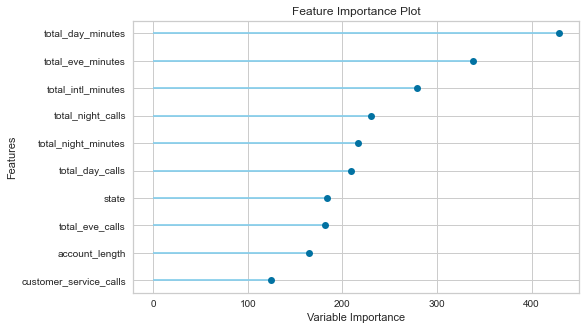

# Feature importance using Shap
interpret_model(final_model, plot = 'summary')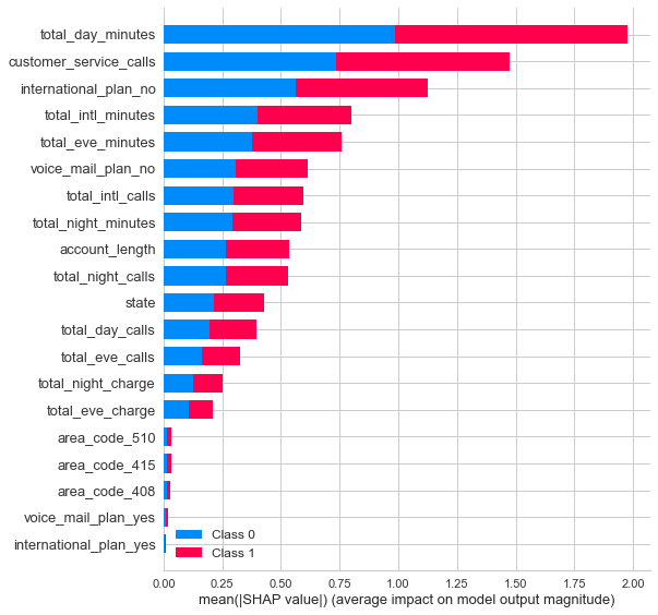

# local interpretation
interpret_model(final_model, plot = 'reason', observation = 14)

Visualization omitted, Javascript library not loaded!
Have you run `initjs()` in this notebook? If this notebook was from another user you must also trust this notebook (File -> Trust notebook). If you are viewing this notebook on github the Javascript has been stripped for security. If you are using JupyterLab this error is because a JupyterLab extension has not yet been written.

# save the model
save_model(final_model,'tuned_lightgbm_dt_save_20201017')

Transformation Pipeline and Model Succesfully Saved

# load the model
loaded_model = load_model('bagged_dt_save_20201017')

Transformation Pipeline and Model Sucessfully Loaded

Potential issues with deploying the model into production are:-

1. Data and model versioning As the amount of data is increasing every day, a mechanism to version data along with code needs to be established. This needs to be done without any cost overhead for storing multiple copies of the same data.
2. Tracking and storing of experiment results and artifacts efficiently. Data scientist should be able to tell which version of model is presently in production, data used for training, what are the evaluation metrics of the model at any given time.
3. Monitoring of models in production for data drift - The behaviour of incoming data may change and will may differ from the data on which it was trained
4. Taking care of CI/CD in production - As soon as a better performing model is finalized and commited, it should go to production in an automated fashion
5. Instead of full-deployment of the models - Canary or Blue-Green deployment should be done. If model should be exposed to 10% to 15% of the population. If it performs well on a small population, then it should be rolled out for everyone.
6. Feedback loops - The data used by the model for prediction going again into the training set

The following tools which can be used for the production issues mentioned above:- 1. Data and model versioning - Data Version Control (DVC) and MLOps by DVC 2. Tracking experiments - mlflow python package 3. Monitoring of models in production - Bi tools 4. Containerization - Docker and Kubernetes 5. CI/CD - Github, CircleCI, MLops 6. Deployment - Seldon core, Heroku 7. Canary / Bluegreen Deployment - AWS Sagemaker

Appendix

If the business priorirty is to predict both churners and non-churners accurately then Accuracy. If the business priority is to identify churners then precision and recall. If the business priority is to predict non-churners (which is a very rare scenario) then it is specificity. The final model will be chosen as per business priority. If the business priority is :- 1. Predicting both churn and non-churning customers accurately then the model with highest accuracy will be chosen i.e - tuned_dt 2. Maximizing the proportion of churner identifications which are actually correct, then model with highest precision - tuned_dt 3. Identifying the Maximum proportion of actual churners then model with highest recall - bagged_dt (as this is simpler than blender_specific)

# Data for DOE
doe = predict_model(loaded_model, data = telecom_churn)
print(metrics.confusion_matrix(doe.churn,doe.Label))

[[2821   29]
 [ 135  348]]

tn, fp, fn, tp = metrics.confusion_matrix(doe.churn,doe.Label).ravel()
Accuracy = round((tp+tn)/(tp+tn+fp+fn),3)
precision = round(tp/(tp+fp),3)
specificity = round(tn/(tn+fp),3)
recall = round(tp/(tp+fn),3)
print( f"Accuracy:{Accuracy} , Specificity:{specificity}, Precision:{precision} , Recall:{recall}")

Accuracy:0.951 , Specificity:0.99, Precision:0.923 , Recall:0.72

doe.shape

(3333, 23)

doe.churn.value_counts()

0    2850
1     483
Name: churn, dtype: int64

93/483

0.19254658385093168